MDWeb Analysis Tutorial
MDWeb provides a friendly environment to analyse your own generated molecular dynamics trajectories. With this short tutorial, you will be able to upload a trajectory and run a set of analysis, checking for example the stability of your system or information about flexibility.
Tutorial Steps
- Registration
- Starting Project
- Uploading a trajectory
- Running Analysis
- Trajectory manipulation: format conversions, slice/snapshot extraction, etc.
- Analysis per Residue/Structure.
- Flexibility Analysis (link to FlexServ).
- Principal Components.
- B-factor landscape.
- Lindemann Coefficients.
- Hinge Point Predictions.
- Residue Correlations.
- etc.
The first thing to do is to choose between working as an anonymous user or alternatively as a registered user. We strongly recommend working as a registered user, as it has some important advantages.
Anonymous user's projects are completely removed once the user is disconnected and also when session expires (after some minutes of inactivity), and therefore working as anonymous user is only suited for a first impression of the web server.
Registration process will just take a minute --> Registration.
Once logged in, the user workspace appears. In this workspace, all projects of the user will be shown.
Now, we are ready to start our first MDWeb analysis project.
MDWeb user can choose between two different kinds of inputs, Simulation and Analysis. In this tutorial, we will see an example of an Analysis project.
You will be asked for a small set of data and input files: First of all, you may fill in a project title and a description (optional) at the top part of the form. Then, at the Input Type drop-down selector, just under the description, you should choose the option Analysis (MD Trajectory). When choosing Analysis as input type, the bottom part of the screen (the one corresponding to Analysis, -Base Trajectory-) will be enabled.

In this example, we are going to compute a set of basic analyes to a 10 ns molecular dynamics simulation of a Serine Hydrolase (pdb code: 1eve). First of all we need to reduce the size of the 10 ns trajectory to be uploaded to MDWeb. In this case, we will just extract 20 snapshots from the original obtained trajectory (one snapshot every 0.5ns). Alternatively, if you wish to have more resolution, you can extract more snapshots by removing solvent molecules, thus drastically reducing the trajectory file size, but to be able to properly analyse this solvent-stripped trajectory, a coherent topology must be generated, and that's usually not an easy job.
Example of reducing trajectory size (click to expand):
XTC Trajectory
Use trjconv from Gromacs package to reduce the size of a trajectory in XTC format.
Usage: trjconv_sp -s structure.gro -f trajectory.xtc -o trajectory.20.xtc -b 1 -e 10000 -dt 500 -ur compact -pbc atom
where structure.gro is the structure topology in GRO format, trajectory.xtc is the trajectory in XTC format, 1-10000 are the starting and ending snapshot times (in ps), and 500 is the offset (write every 500 ps). The rest of the commands are useful when dealing with non-cubic boxes (-ur) and periodic boundary conditions (-pbc).
You will be asked for a group to write to the output file, e.g.:
Will write xtc: Compressed trajectory (portable xdr format)
Select group for output
Opening library file /usr/local/gromacs/share/gromacs/top/aminoacids.dat
Group 0 ( System) has 99637 elements
Group 1 ( Protein) has 8380 elements
Group 2 ( Protein-H) has 4263 elements
Group 3 ( C-alpha) has 534 elements
Group 4 ( Backbone) has 1602 elements
etc.
We are going to choose System (group 0), to write all the system as output and hence being coherent with the system topology.
Executing these commands will generate a new trajectory with 20 snapshots (10000/500), named trajectory.20.xtc, in Gromacs XTC format, ready to be uploaded to MDWeb server.
Use ptraj from Ambertools package to reduce the size of a trajectory in DCD, NetCDF, Binpos or CRD formats.
Usage: ptraj structure.top < ptrajReducing.in
where structure.top is the structure topology in PRMtop or PSF format, and ptrajReducing.in is a file containing the apropriate commands:
trajin trajectory.crd 1 10000 500 # Input trajectory, first and last snapshot to read and offset.
trajout trajectory.20.crd # Output trajectory, in Amber ASCII CRD format (ptraj default).
go
Executing these commands will generate a new trajectory with 20 snapshots (10000/500), named trajectory.20.crd, in Amber ASCII CRD format, ready to be uploaded to MDWeb server.
To start our analysis, we are going to put this new generated 20 snapshots trajectory in the Trajectory File input box, and the associated topology (the same file used for the molecular dynamics simulation) in the Topology File input box.

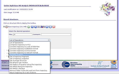
Once we have our trajectory uploaded, we can begin with the analysis. MDWeb offers a set of basic analysis that can be divided in 3 different sections:
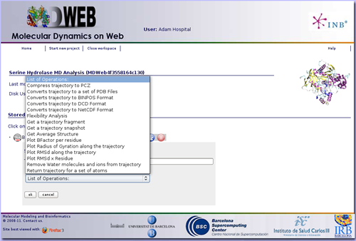
In this specific example we are not interested in converting the trajectory format, but we will begin applying some manipulations to it. The most usual and important one is stripping the solvent, usually toghether with the counterions, when user is only interested in studying the protein molecule.
To do that, click on the operation called Remove water molecules and ions from trajectory. We can choose whether we would like to remove only water molecules, only counterions or both. In this case, we will remove both, obtaining the trajectory (and the correct topology associated) for just the structure of interest.

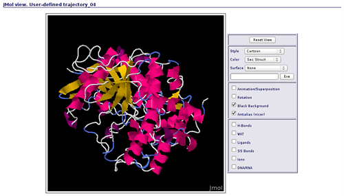
The first noticeable thing once we have the "dry" trajectory, is that it is really smaller in size than the solvated one. That allows the user to animate the trajectory with JMol applet. If we try to visualize the original solvated structure, MDWeb will show a warning message because the trajectory is too large, recommending to remove solvent. So, clicking at the corresponding JMol icon ![]() , a new window with the JMol interactive visualizer will be opened. It is a good first aproximation to take a look at the dynamics of the structure, before obtaining analysis data.
, a new window with the JMol interactive visualizer will be opened. It is a good first aproximation to take a look at the dynamics of the structure, before obtaining analysis data.
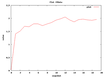
Now we can begin with the basic data analysis. From the list, we can choose two basic analysis as Root Mean Square deviation and Radius of Gyration. With these two analysis we will be able to see the deviation of the structure during the dynamics, whether it maintains its conformation during the 10 ns length or it suffers some distortion.
Each of the analysis plot can be visualized clicking at the correspondent icon ![]() .
.
 |
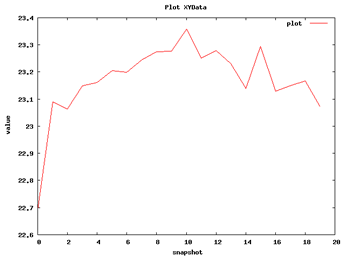 |
| RMSd Analysis | Radius of Gyration |
We can apply a couple of additional analysis to get a first impression about the flexibility of the structure. These are the Root Mean Square deviation per Residue and the Bfactor per Residue analyses. Taking a look at the plots, we can easily identify the regions of the structure having more mobility (usually loops) and the regions that are almost kept fixed during the whole simulation.
 |
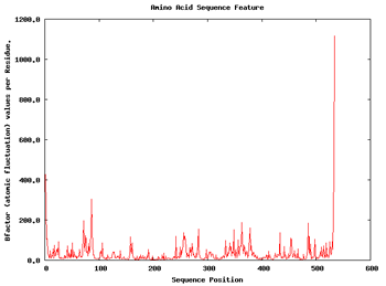 |
| RMSd x Residue | Bfactor x Residue |
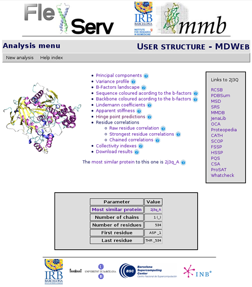
If we are interested in more flexibility analysis, MDWeb offers the possibility to send the project to our flexibility server FlexServ. Just click on the operation called Flexibility Analysis.
FlexServ is a server aimed to show in an easy and visual way flexibility-related properties of proteins. It computes a big set of flexibility analysis like:
So with this set of analysis, we have been able to see that the simulated structure has not suffered critical structural deformations. It has not gone more than 2Å away from the initial structure, and the Radius of Gyration has been also maintained around 20Å. From the flexibility part, we identified some flexible regions from the Bfactor and RMSd per residue analysis, that are located mostly in loop regions. We launched a FlexServ analysis to obtain more information about these flexible parts.