Normal Mode Analysis (NMA) can be defined as the multidimensional treatment of coupled oscillators from the analysis of force-derivatives in equilibrium conformations. This methodology assumes that the displacement of an atom from its equilibrium position is small and that the potential energy in the vicinity of the equilibrium position can be approximated as a sum of terms that are quadratic in the atomic displacements. In its purest form, it uses the same all-atom force field from a MD simulation, implying a prior minimization in vacuo (Go and Scheraga 1976; Brooks III, Karplus et al. 1987). Tirion (1996) proposed a simplified model where the interaction between two atoms was described by Hookean pairwise potential where the distances are taken to be at the minimum, avoiding the minimization (referred as Elastic Network Model). This idea being further extended to use coarse-grained (Cα) protein representation by several research groups, as in the Gaussian Network Model (Bahar et al. 1997; Haliloglu et al. 1997). The GNM model was later extended to a 3-D, vectorial Anisotropic Network Model, which is the formalism implemented in our server (Atilgan et al. 2001). Through the diagonalization of the hessian matrix, the ANM provides eigenvalues and eigenvectors that not only describe the frequencies and shapes of the normal modes, but also their directions.

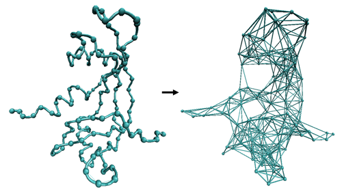
Within the elastic network model approach (ENM) the network topology is described by a Kirchhoff matrix Γ of inter-atomic contacts where the ij-th element is equal to -1 if nodes (i.e., Cα) i and j are within the cutoff distance r_c, and zero otherwise, and the diagonal elements (ii-th) are equal to the connectivity of the residue:

$\Gamma_{ii}=\sum_{k|k\neq i}^N{\Gamma_{ik}}$

(1)

In the ANM approach, the potential energy between two residues i-j is given by:

$E=0.5\cdot \gamma\cdot\Gamma_{ij}\left(r_{ij}-r_{ij}^0\right)^2$

(2)

where r_ij and r_ij⁰ are the instantaneous and reference (equilibrium) position vectors of atoms i and j and γ is the force constant; in the original formalism by Atilgan et al, γ=1 kcal/mol.Å² (see below).

For the sake of simplicity, the product of the force constant for a given i, j pair γ_ij and the corresponding Kirchhoff matrix element Γ_ij can be expresed as a single stiffness constant K_ij:

$K_{ij}=0.5\cdot\gamma\cdot\Gamma_{ij}$

(3)

The molecular Hamiltonian is given by the elastic energy to displace a protein from its equilibrium conformation:

$E=\sum_{i\neq j}{K_{ij}\left(r_{ij}-r_{ij}^0\right)^2}$

(4)

This potential function is used to build a Hessian matrix (H), a 3N x 3N matrix (N is the number of nodes in the protein) defined as N x N submatrices H_ij containing the second derivatives of the energy respect the coordinates of each protein node. Diagonalization of the Hessian yields the eigenvectors (the essential deformation modes) and the associated eigenvalues (stiffness constants).

As presented, NMA defines springs between all pairs of residues with no zero elements in the corresponding Kirchhoff matrix element Γ_ij. In principle all inter-residue force-constants have then two possible values 0 if the residues are not connected (Kirchhoff matrix element equal to 0) and γ otherwise. The standard approach (Tirion 1996) defines the connectivity index by using an spherical cutoff r_c:

$\Gamma_{ij}=-1$ if $r_{ij}^{0}\leq r_c$ and $\Gamma_{ij}=0$ otherwise.

(5)

Cutoff distances around 8-12 Å have been used, being the most usual the range 8-9 Angstroms, but some authors exploring values as high as 20-25 Å (Sen & Jernigan, 2006). Different cut-off radii can be used for different proteins based on size, shape, density or other protein characteristics (Orellana et al., to be published).

Regarding the force constant parameter γ, many authors set values equal to 1, which means that eigenvectors have physical sense, but eigenvalues are not realistic. Alternatively, γ can be fitted to reproduce X-ray B-factors or MD simulation results.

This approximation, with interactions defined by an uniform γ within a cutoff, is referred to as distance cutoff, and despite its simplicity provides good descriptions of large-scale molecular motions (Bahar and Rader, 2005; Ma, 2005). However, the use of an empirical cutoff, though useful to eliminate irrelevant interactions and explore topological constraints in equilibrium dynamics, introduces a sharp discontinuity in the Hamiltonian and some degree of arbitrareness and uncertainty in the method. Other approaches have been developed to define continuum functions for the spring constant. Kovacs et al. (2004) developed a simple function that assumes an inverse exponential relationship between the distance and the force-constant:

$K_{ij}=C\left(\frac{r^{*}}{r_{ij}^0}\right)^6+as_{ij}$

(6)

where C is a stiffness constant (taken as 40 kcal/mol Å²), r^* is a fitted constant, taken as the mean Cα-Cα distance between consecutive residues (3.8 Angstroms), r_ij⁰ is the equilibrium distance between the Cα of residues i and j and as_ij is a inter-residue residue constant surface. In practice, the surface correction is small and has been ignored in our implementation of the method, which is available in FlexServ as an alternative to standard cutoff-based method. This method maintains the simplicity of the original method and avoids the problems intrinsic to the use of a cutoff. The major drawback is that, by connecting all residues in the network, both increases the rigidity of the system and lowers the speed of the computation.

We have recently improved cutoff-based and Kovac’s versions of NMA by a multi-parametric fitting of NMA to atomistic MD simulations in a large number of proteins (Orellana et al., to be published). The refined method, which is available in FlexServ defines a network topology by an effective Kirchhoff matrix Γ that is the sum of a Rouse Chain topology matrix for the first 3 neighbours, with a usual Kirchhoff matrix for distant interactions, rendering a mixed connectivity matrix that combines both sequential and distant information. Thus, given a pair of residues i, and j with sequential distance S_ij>0 and Cartesian distance r_ij, the ij-th element of the inter-residue contact matrix is defined as:

$\Gamma_{ij}=\left\{\begin{matrix} S_{ij}<3, & \Gamma_{ij}=-1 \\ S_{ij}>3, & \left\{\begin{matrix} \Gamma_{ij}=-1 & if\; r_{ij}^0 \leq r_{c}\\ \Gamma_{ij}=0 & otherwise \end{matrix} \end{matrix}\right. }}$

(7)

The distance (both in Cartesian and Sequence space) dependence of the force-constant, and the associated scaling factors C_cart and C_seq (eq.8) were adjusted to reproduce atomistic MD simulations (C_seq=60 kcal/mol.Å² and C_cart=6 kcal/mol.Å², lower or higher values can be considered for extremely small or large systems). The same fitting procedure was followed to obtain a size-dependent cutoff distance (r_c), that can be approximated with a logarithmic function of the protein lenght, with extreme values of 8 and 16 Angstroms for most proteins (up to 17-20 Angstroms for extremely large proteins, above 700 residues). Thus the MD-ANM mixed model combines an MD calibrated inverse exponential function with a lenght-dependent cutoff to discard redundant interactions, also improving computational efficency. The resulting network gives flexibility patterns closest to MD, being not only the eigenvectors, but also the eigenvalues more physically meaningful.

Our FlexServ implements the ANM formalism with the three different definitions of the force constants described above:

The so called linear or distance-cutoff formalism, equal to the original ANM but with a default γ=10 kcal/mol.Å² for the ANM linear implementation as in ElNémo (Suhre & Sanejouand (2004)). The default cutoff value in this case is 8Å, or 9Å for larger proteins (above 150-200 residues).
The Kovacs, inverse exponential formalism, in which the force constant is defined by a continuous function; the default values of C=40 kcal/mol Å², and r_ij⁰=3.8 Å is used; as_ij term is neglected
The Mixed formalism, in which the force constant follows a complex definition with all parameters (r_c, C_cart and C_cont) fitted according to MD simulations as explained before:

$K_{ij}\left\{\begin{matrix}&space;S_{ij}\leq&space;3,&space;&&space;K_{ij}=\frac{C_{seq}}{S_{ij}^2}&space;\\&space;S_{ij}>3,&space;&&space;\left\{\begin{matrix}K_{ij}=\left(\frac{C_{cart}}{r_{ij}^0}\right)^6&if\;r_{ij}^0\leq&space;r_{c}\\&space;K_{ij}=0&space;&&space;otherwise&space;\end{matrix}\right.&space;\end{matrix}\right.&space;}}$

(8)

Note that once NMA is performed and the set of eigenvectors/eigenvalues is determined, Cartesian pseudo-trajectories at physiologic temperature can be obtained by activating normal mode deformations using a Metropolis Monte Carlo algorithm with a Hamiltonian defined as shown in eq. 9. The displacements obtained by such algorithm can then be projected to the Cartesian space to generate “pseudo-trajectories”. Note that by limiting the size of the sum in eq. 9 to only important eigenvectors (m’<n) trajectory can be enriched in sampling of essential deformation modes (Rueda et al. 2007a).

$E=\sum_{i=1}^{m^\prime}{K_i\Delta D_i^2}$

(9)

where $K_i=\frac{k_BT}{2\lambda}$ (λ being the eigenvalue in distance² units) and ΔD_i is the displacement along the mode.