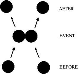
In this approach (Alder and Wainwright,1959; Emperador et al. 2008) the proteins are modelled as a system of beads (Cα atoms) interacting through a discontinuous potential (square wells in our study). Outside the discontinuities, potentials are considered constant, thereby implying a ballistic regime for the particles (constant potential, constant velocity) in all conditions, except at such time as when the particles reach a potential discontinuity (this is called “an event” or “a collision”). At this time, the velocities of the colliding particles are modified by imposing conservation of the linear momentum, angular momentum, and total energy. Since the particles were constrained to move within a configurational space where the potential energy is constant (infinite square wells), the kinetic energy remains unchanged and therefore all collisions are assumed to be elastic.
DMD has a major advantage over techniques like MD because, as it does not require the integration of the equations of motion at fixed time steps, the calculation progresses from event to event. In practice, the time between events decreases with temperature and density and depends on the number of particles N approximately as N-1/2. The equations of motion, corresponding to constant velocity, are solved analytically
where tc is the minimum amongst the collision times tij between each pair of particles i and j, given by
where rij is the square modulus of , vij is the square modulus of
,
, and
is the distance corresponding to a discontinuity in the potential (the signs + and - before the radical are used for particles approaching one another and moving apart, respectively).
As the integration of Newton’s equations is no longer the rate limiting step, calculations can be extended for very long simulation periods and large systems (Peng et al , 2004, Ding et al. 2005, Sharma et al. 2007) provided an efficient algorithm for predicting collisions is used (Smith et al. 1997).
The collision between particles i and j is associated with a transfer of linear momentum in the direction of the vector . Thus,
where the prime indices variables after the event.
To calculate the change in velocities, the velocity of each particle is projected in the direction of the vector so that the conservation equations become one-dimensional along the interatomic coordinate
which implies
From Eqs. 5-8 the transferred momentum is readily determined as
and the final velocities of particles i and j are determined through Eqs. 3 and 4.
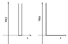
The interaction potentials are defined as infinite square wells, such that the particle-particle distances vary between dmin=(1-σ)rij0 and dmax=(1+σ)rij0, rij0 being the distance in the native conformation and 2σ the width of the square well. The MD-averaged conformation was taken as the native conformation. Residue-residue interaction potentials are defined only for the particles at a distance smaller than a cut-off radius rc in the native conformation (left figure above). Otherwise the particles only interact via a hardcore repulsive potential that avoids steric clashes (right figure above). For non-consecutive Cα particles, rc = 8 Å and σ = 0.1 were used, while for consecutive pairs of residues a smaller well width (σ = 0.05) was chosen to keep the Cα – Cα distances closer to the expected value: 3.8 Å.