FlexServ tutorial

Welcome to the "first steps" tutorial. In this small document you will learn how to start using this tool to perform your own analysis about flexibility on proteins.

In the first place, you need to get a PDB file with the protein that you want to analyze. We will use the Protein Data Bank web to get a file with this format. For this tutorial we will choose a protein which PDB code is 1B9P. Type "1B9P" in the search box and hit enter. You will arrive to a page that contains the information about the protein. We are interested in the download link to get the PDB file.

Once we have the PDB file, we can open the FlexServ web tool and prepare the analysis. Near the end of the page, you will see a form like this:

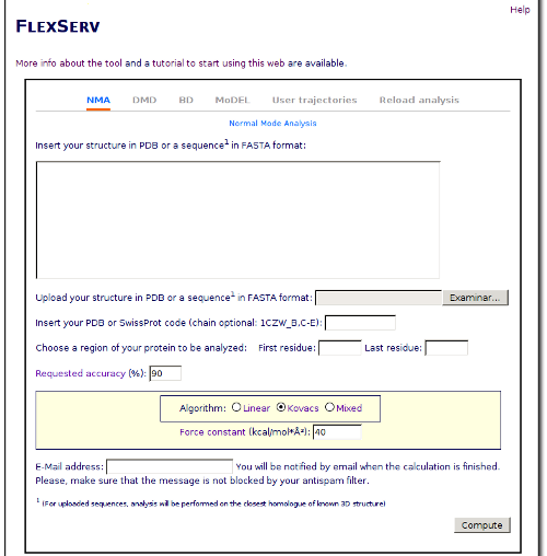
In this form, we will put the downloaded file in the box labeled "Upload your structure in PDB format". Now that we have choosen which structure will be the starting point, we have to choose the kind of simulation that we want to perform. In this tutorial, we will perform a simulation using the Brownian Dynamics simulator. Click on the BD radio button, and the options for this kind of simulation will appear just below:

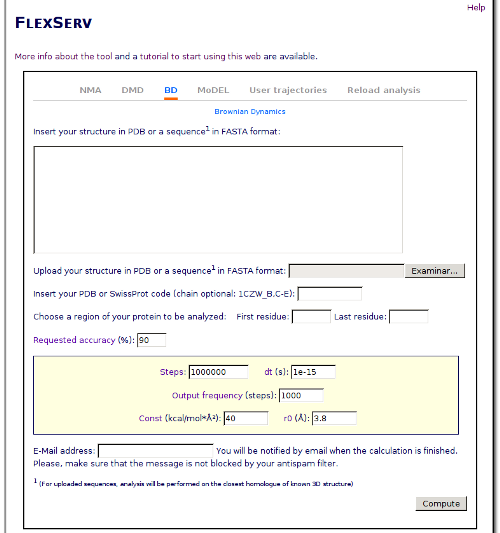
The protein choosen is not a big one, so we will not change the number of steps that we will perform and will stick to the default values. Anyway, you can change the number of steps, the time step or the output frequency if you desire to experiment with the parameters.

It is always recommended that you introduce your e-mail address in the box below. If the tool has your e-mail address, it will send you a mail when the calculation finish. In that way, you can forget about it until it is finished, and no data will be lost if you lose your internet connection.

Finally, click on the Compute button to start the calculation. This simulation will take a couple of minutes.

Once the simulation and further analysis are performed, the results page are shown:

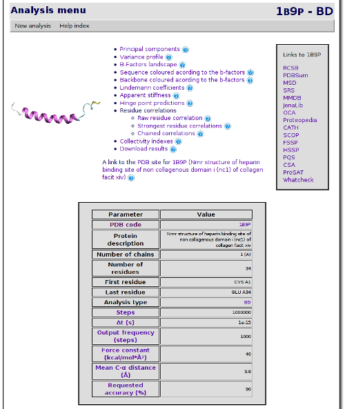
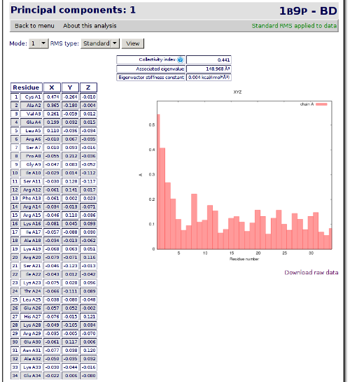
From this point, you can browse the results freely, navigating through the different pages. But I will explain how to perform and use some of the analysis available. We will start with a basic view of the eigenvectors. Click on Principal Components link. A page showing the principal components and some related graphics is shown:

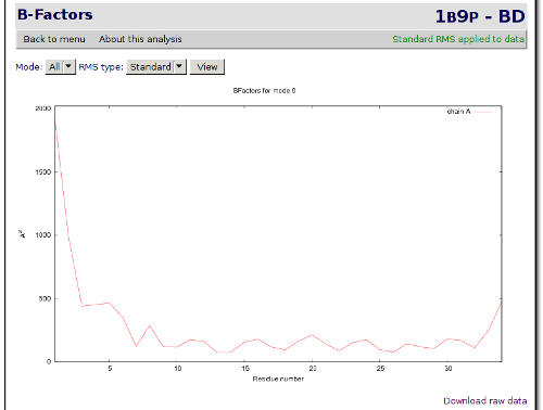
Next we will go back to the analysis index page clicking on the Back to menu link, in the top-left area of the analysis page. The next analysis that we will check is the B-factors landscape. Click on the B-factors landscape link to check the temperature factor and the mobility of the residues.

After having checked the basic analysis, we will jump now to a more complex one. We will start with a correlation analysis. Click on the Back to menu link to return to the index and then on Strongest correlations per residue link to go to the analysis. It brings you to a page where each residue shows which other residue have the higher positive correlation and which residue have the higher negative correlation.

In this analysis you will see that most of the correlations are trivial: one residue is correlated with the next in the sequence. To filter this kind of residues you can choose Distance from the drop-down list, write 10 at the Minimum distance text box and click on View. The data is recomputed at the server, and a new set of residues is shown. This time, the residues are farther than the distance choosen in the Minimum distance text box. In this way, we are excluding correlations from residues that are too near to be interesting.

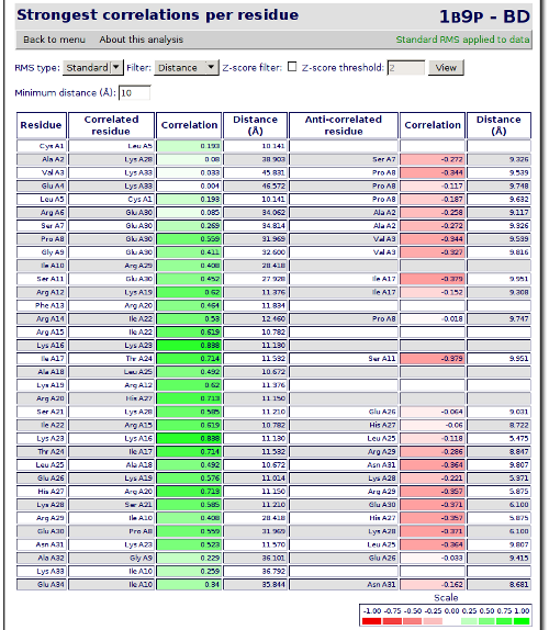
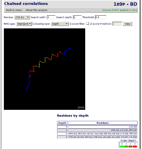
With this data, we can see than residue 16 has a quite high correlation with residue 23. Now we are going to see which are the residues more correlated to residue number 16. Click on the Back to analysis selection at the end of the page and then go to Chained correlations. This analysis allows you to enter a starting residue and perform a search for the more correlated residues of this one in different depths. For the analysis that we want to perform, we will select the residue number 16 at the Residue combo, 3 at the Search width one and 3 at the Search depth text box. Now click on View.

The page is reloaded, but this time, the JMol applet shows the residues that has been found correlated highlighted in colors (a gradient from green to red):

This is an example of the different analysis that can be performed with this tool. Now, feel free to try the other different options. All of them work in a similar way and offer a lot of possibilities.

Enjoy!