Despite recent advances in experimental techniques, the study of flexibility is mostly a task for theoretical methods. The most powerful of them is atomistic molecular dynamics (MD, McCammon, et al., 1977), a rigorous method with solid physical foundations, which provides accurate representations of protein flexibility under physiological-like environments. Unfortunately, despite its power, MD are complex, computationally expensive and their use requires a certain degree of expertise (Karplus and Kuriyan, 2005; Rueda, et al., 2007b). The alternative to atomistic MD is the use of coarse-grained methods coupled to simple potentials (Tirion, 1996; Dokholyan, et al., 1998). By using these techniques we assume a lost of atomic detail to gain formal and computational simplicity in the representation of near-native state flexibility of proteins (Ma, 2005; Rueda, et al., 2007a ; Emperador, et al., 2008). Unfortunately, despite its power, the practical use of coarse-grained methods is still limited, due mostly to the lack of standardized protocols for analysis and the existence of a myriad of different algorithms distributed in different websites.

We present here FlexServ, an integrated tool that tries to link most important coarse-grained based methods, structural databases, and atomistic models with a powerful analysis platform. FlexServ incorporates three coarse-grained algorithms for the representation of protein flexibility: i) Discrete dynamics (DMD), ii) Normal mode analysis (NMA) based on different types of elastic networks and iii) Brownian dynamics (BD). The first technique (DMD) assumes that residue-residue interactions are controlled by infinite square wells centered at equilibrium distance with width fitted to reproduce atomistic flexibility (Emperador, et al., 2008). Within this approach a Cα is either moving at constant velocity or colliding elastically with a wall, which allows the derivation of trajectories using simple ballistic equations without integration of Newton’s equations of motion (for discussion see Emperador, et al., 2008). On the other hand, elastic NMA and BD assume that inter-residue interactions are controlled by a harmonic-like potential energy expressed as:

$E_{ij}=\delta_{ij}K_{ij}\left(r_{ij}^0\right)\left(r_{ij}-r_{ij}^0\right)^2$

(1)

where r_ij is the distance between residues i and j, and r_ij⁰ the equilibrium value, Γ_ij the Kirkchoff connectiviy matrix, and K_ij(r_ij⁰) the stiffness force constant. In a pure harmonic model K_ij(r_ij⁰) takes a single value K_ij and Γ_ij=-1 for atoms within a given cutoff and 0 otherwise. In Kovacs' pseudo-harmonic model (2004), K_ij(r_ij⁰) has a (1/r_ij⁰)⁶ dependence (Kovacs, et al., 2004) and no cutoff is applied. FlexServ incorporates both Hamiltonian definitions as well as a new hybrid one (Orellana, L.; et al. unpublished) which treats differently covalently bonded and non-bonded residues and that is fitted to reproduce atomistic MD results.

Approximation of a potential with an harmonic function

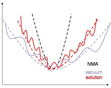
NMA (within the Anisotropic Network Model formalism (Altigan, et al 2001)) uses the energy function to define the Hessian whose diagonalization provides the eigenvectors and eigenvalues characterizing the harmonic deformability of the protein. NMA based pseudo-trajectories are generated by activating movements along the eigenvectors using a Metropolis-Monte Carlo algorithm (Rueda, et al., 2007a). Within the BD approach the energy functional is used to compute forces, which are fed into a Brownian algorithm, which computes trajectories using standard defaults for integration, friction and Stochastic terms (see Emperador, et al., 2008 for details).

FlexServ incorporates a large variety of methods to characterize flexibility. Thus, the server performs basic analysis like structural oscillation using root mean square deviation (RMSd) or a gaussian RMSd (gRMSd) algorithm, which fits the molecules reinforcing the alignment of rigid moieties and favoring the location of movements into flexible regions. Essential dynamics routines (Amadei, et al., 1993) are used to characterize most important deformation modes are obtained by diagonalization of the trajectory covariance matrix. The eigenvectors represent the nature of the essential deformation patterns, while the eigenvalues can be transformed into the frequencies or stiffness of these movements. Essential deformation movements (after either rmsd or rrmsd fitting) are ranked by importance and can be visualized and processed to obtain information (see Meyer, et al., 2006; Rueda, et al., 2007a for a detailed explanation), such as B-Factor profiles, the “collectivity” index (a measure of the collective nature of protein motions, Brüschweiler, 1995), the variance profile, the dimensionality (the number of movements defining a percentage of variance), or the size of the essential space (the number of modes with eigenvalues > 1 Å²). Lindemann’s indexes are computed to evaluate the liquid/solid nature of the entire or partial regions of the protein (Rueda, et al., 2007b; Zhou, et al., 1999).

Advanced capabilities of FlexServ include calculation of the apparent stiffness between interacting residues (obtained by inverting the inter-residue covariance, Rueda, et al., 2007a) and the determination of residue-correlations using different algorithms that allow the user to filter non-relevant or spurious correlations.

Other advanced tools allow the determination of dynamic domains and hinge points using a variety of techniques: i) exploration of the B-factor landscape after fitting with the gRMSd method, ii) analysis of the force-constant profile (Sacquin-Mora and Lavery, 2006) and iii) clustering by inter-residue correlation (Navizet, et al., 2004). Calculations are performed using different sliding windows to reduce noise and false positives.

In all the analysis data are presented as plain text, or 2D plots or shown on the 3D structure when appropriate.

Introduction