ABC MD Setup pipeline using BioExcel Building Blocks (biobb)
ABC MD Setup pipeline using BioExcel Building Blocks (biobb)
This BioExcel Building Blocks library (BioBB) workflow provides a pipeline to setup DNA structures for the Ascona B-DNA Consortium (ABC) members. It follows the work started with the NAFlex tool to offer a single, reproducible pipeline for structure preparation, ensuring reproducibility and coherence between all the members of the consortium. The NAFlex pipeline was used for the preparation of all the simulations done in the study: The static and dynamic structural heterogeneities of B-DNA: extending Calladine–Dickerson rules. The workflow included in this Jupyter Notebook is extending and updating the NAFlex pipeline, following the best practices exposed by the Daniel R. Roe and Bernard R. Brooks work, and is being used for the new ABC study.
The setup process is performed using the biobb_amber module from the BioBB library, which is wrapping the AMBER MD package. The forcefield used is the nucleic acids specific parmbsc1 forcefield, with Joung & Cheatham monovalent ion parameters for Ewald and TIP4P/EW water and SPC/E Water model.
The main steps of the pipeline are:
- Generate structure topology
- Solvate structure with a truncated octahedron box, with SCP/E water model
- Neutralize the system with Potassium ions
- Add an ionic concentration of 150mM of Cl- / K+ ions
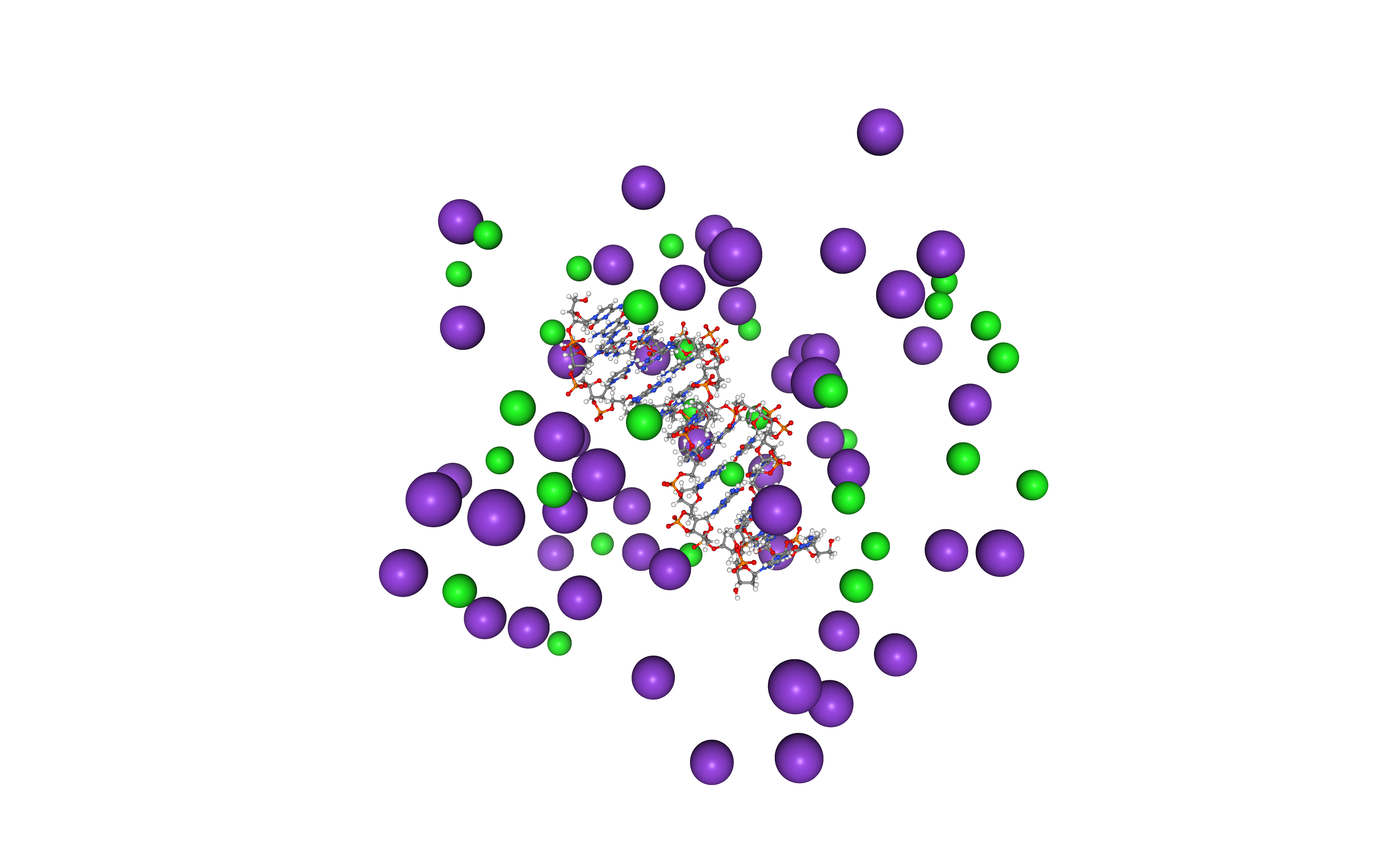
- Randomize ions around the structure using cpptraj
- Generate H-mass repartitioned topology to run the production simulations with a 4fs timestep
- Equilibrate the system in solvent with a 10-steps protocol (Daniel R. Roe and Bernard R. Brooks)
- Production Run (4fs timestep)
Settings
Biobb module used
- biobb_amber: Tools to setup and run Molecular Dynamics simulations using the AMBER MD package.
Auxiliary libraries used
- jupyter: Free software, open standards, and web services for interactive computing across all programming languages.
- plotly: Python interactive graphing library integrated in Jupyter notebooks.
- nglview: Jupyter/IPython widget to interactively view molecular structures and trajectories in notebooks.
- simpletraj: Lightweight coordinate-only trajectory reader based on code from GROMACS, MDAnalysis and VMD.
- gfortran: Fortran 95/2003/2008/2018 compiler for GCC, the GNU Compiler Collection.
- libgfortran5: Fortran compiler and libraries from the GNU Compiler Collection.
Conda Installation
git clone https://github.com/bioexcel/biobb_wf_amber.git
cd biobb_wf_amber
conda env create -f conda_env/environment.yml
conda activate biobb_wf_amber
jupyter-notebook biobb_wf_amber/notebooks/abc_setup/biobb_wf_amber_abc_setup.ipynb
Pipeline steps
- Initial Parameters
- Generate Topology
- Add Water Box
- Adding additional ionic concentration
- Randomize Ions
- Generate Topology with Hydrogen Mass Partitioning (4fs)
- System Equilibration
- Free MD Simulation
- Output files
 |
 |
Initializing colab
The two cells below are used only in case this notebook is executed via Google Colab. Take into account that, for running conda on Google Colab, the condacolab library must be installed. As explained here, the installation requires a kernel restart, so when running this notebook in Google Colab, don't run all cells until this installation is properly finished and the kernel has restarted.
# Only executed when using google colab
import sys
if 'google.colab' in sys.modules:
  import subprocess
  from pathlib import Path
  try:
    subprocess.run(["conda", "-V"], check=True)
  except FileNotFoundError:
    subprocess.run([sys.executable, "-m", "pip", "install", "condacolab"], check=True)
    import condacolab
    condacolab.install()
    # Clone repository
    repo_URL = "https://github.com/bioexcel/biobb_wf_amber.git"
    repo_name = Path(repo_URL).name.split('.')[0]
    if not Path(repo_name).exists():
      subprocess.run(["mamba", "install", "-y", "git"], check=True)
      subprocess.run(["git", "clone", repo_URL], check=True)
      print("⏬ Repository properly cloned.")
    # Install environment
    print("⏳ Creating environment...")
    env_file_path = f"{repo_name}/conda_env/environment.yml"
    subprocess.run(["mamba", "env", "update", "-n", "base", "-f", env_file_path], check=True)
    print("🎨 Install NGLView dependencies...")
    subprocess.run(["mamba", "install", "-y", "-c", "conda-forge", "nglview==3.0.8", "ipywidgets=7.7.2"], check=True)
    print("👍 Conda environment successfully created and updated.")
# Enable widgets for colab
if 'google.colab' in sys.modules:
  from google.colab import output
  output.enable_custom_widget_manager()
  # Change working dir
  import os
  os.chdir("biobb_wf_amber/biobb_wf_amber/notebooks/abc_setup")
  print(f"📂 New working directory: {os.getcwd()}")
import nglview
import ipywidgets
import plotly
import sys
import plotly.graph_objs as go
Initial parameters
Input parameters needed:
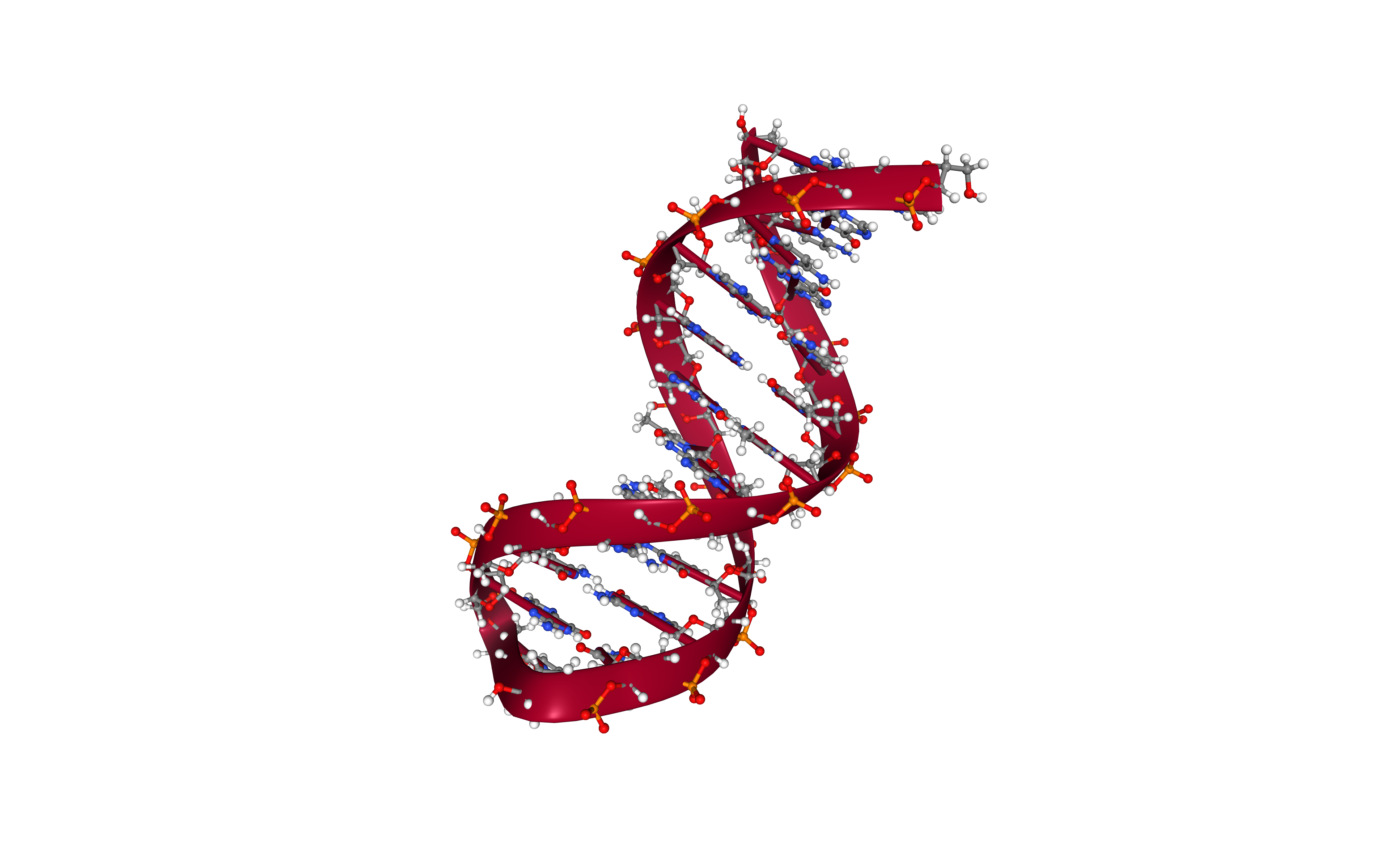
- DNA file: DNA pdb file prepared for a MD simulation (e.g. GCGCGGCTGATAAACGAAAGC)
- Forcefield: Forcefield to be used in the setup (e.g. protein.ff14SB).
- Water model: Water model to be used in the setup (e.g. SPC/E).
- Ion model: Ion model to be used in the setup (e.g. Dang).
- Thermostat: Thermostat to be used in the setup (e.g. Langevin).
- Timestep: Simulation timestep (e.g 2fs).
dna_pdb = "CGCGAATTCGCG.pdb" # Drew-Dickerson dodecamer
forcefield = ["DNA.bsc1"] # ParmBSC1 (ff99 + bsc0 + bsc1) for DNA. Ivani et al. Nature Methods 13: 55, 2016
water_model = "OPCBOX" # SPC/E + Joung-Chetham monovalent ions + Li/Merz highly charged ions (+2 to +4, 12-6 normal usage set)
ions_model = "ionsjc_tip4pew" # Monovalent ion parameters for Ewald and TIP4P/EW water from Joung & Cheatham JPCB (2008)
# Show protein
view = nglview.show_structure_file(dna_pdb)
view.add_representation(repr_type='ball+stick', selection='all')
view._remote_call('setSize', target='Widget', args=['','600px'])
view
Generate Topology
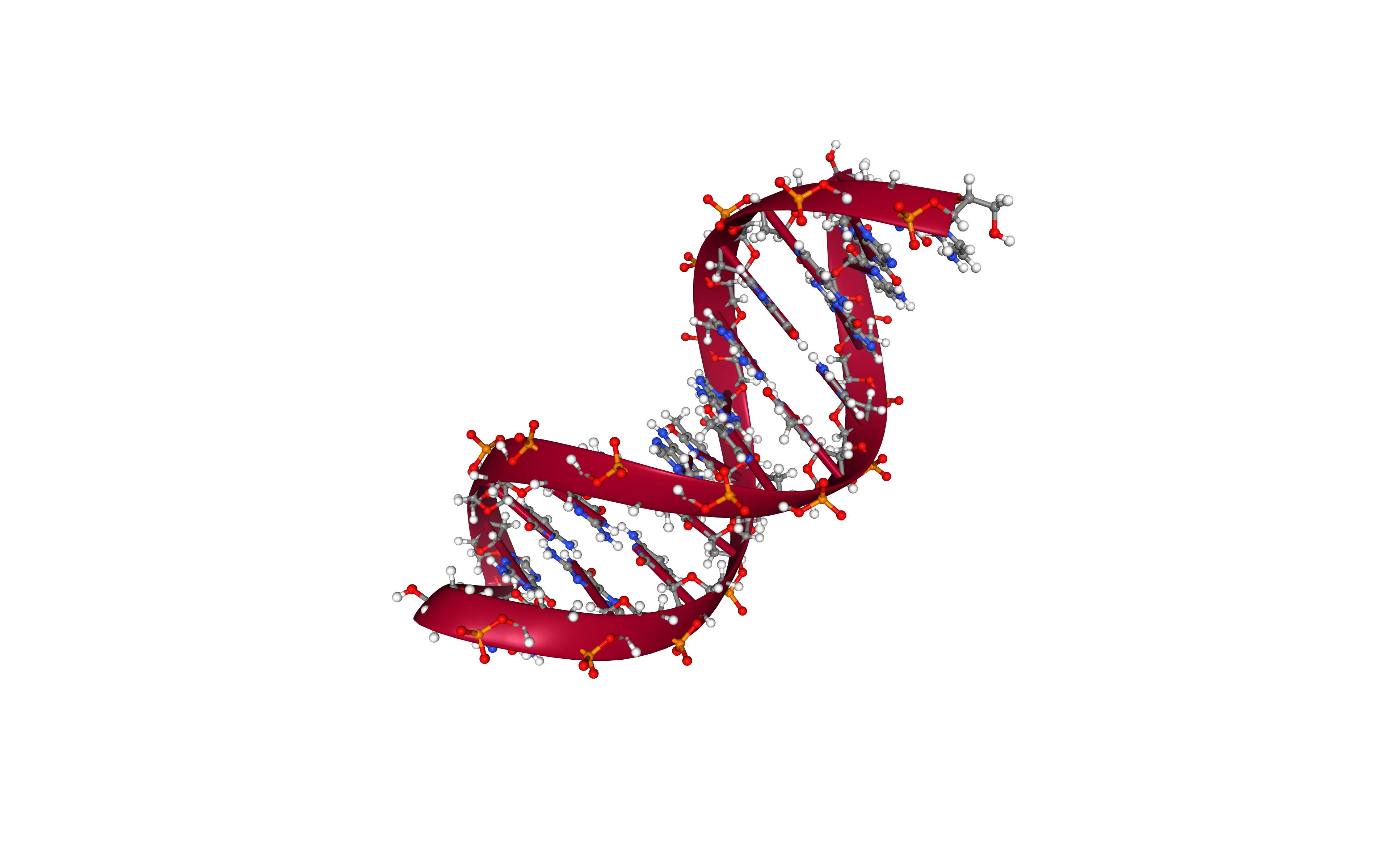
Build the DNA topology from the modelled structure using the leap tool from the AMBER MD package.
Using the forcefield fixed in the first cell.
Building Blocks used:
- leap_gen_top from biobb_amber.leap.leap_gen_top
# Import module
from biobb_amber.leap.leap_gen_top import leap_gen_top

# Create prop dict and inputs/outputs
prop = {
    "forcefield" : forcefield
}
dna_leap_pdb_path = 'structure.leap.pdb'
dna_leap_top_path = 'structure.leap.top'
dna_leap_crd_path = 'structure.leap.crd'

# Create and launch bb
leap_gen_top(input_pdb_path=dna_pdb,
           output_pdb_path=dna_leap_pdb_path,
           output_top_path=dna_leap_top_path,
           output_crd_path=dna_leap_crd_path,
           properties=prop)
# Show protein
view = nglview.show_structure_file(dna_leap_pdb_path)
view.add_representation(repr_type='ball+stick', selection='all')
view._remote_call('setSize', target='Widget', args=['','600px'])
view
Adding Water Box
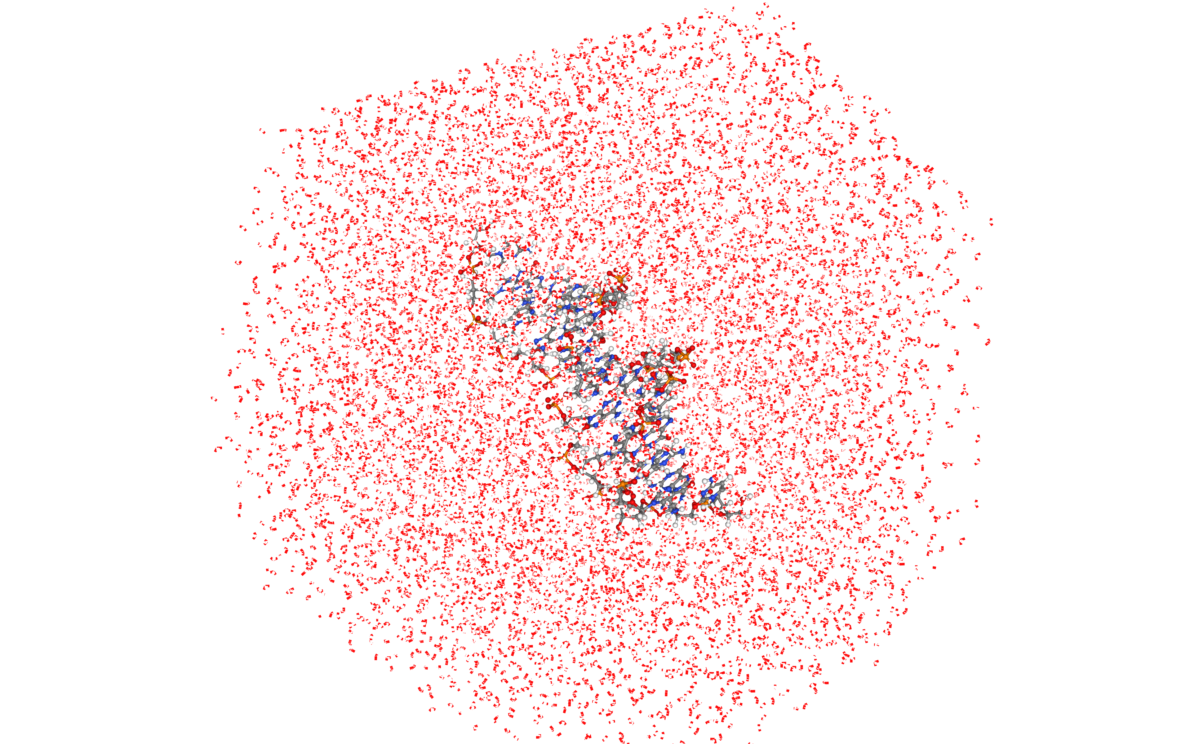
Creating a water box surrounding the DNA structure using the leap tool from the AMBER MD package.
Using the water model fixed in the first cell.
Building Blocks used:
- amber_to_pdb from biobb_amber.ambpdb.amber_to_pdb
- leap_solvate from biobb_amber.leap.leap_solvate
# Import module
from biobb_amber.leap.leap_solvate import leap_solvate

# Create prop dict and inputs/outputs
prop = {
    'forcefield': forcefield,
    'water_type': water_model,
    'ions_type' : ions_model,
    'box_type': 'truncated_octahedron',
    'distance_to_molecule' : 15.0,
    'neutralise' : True,
    'iso' : True,
    'closeness' : 0.97,
    'positive_ions_type' : "K+"
}

output_solv_pdb_path = 'structure.solv.pdb'
output_solv_top_path = 'structure.solv.parmtop'
output_solv_crd_path = 'structure.solv.crd'

# Create and launch bb
leap_solvate( input_pdb_path=dna_leap_pdb_path,
            output_pdb_path=output_solv_pdb_path,
            output_top_path=output_solv_top_path,
            output_crd_path=output_solv_crd_path,
            properties=prop)
# Show protein
view = nglview.show_structure_file(output_solv_pdb_path)
view.clear_representations()
view.add_representation(repr_type='ball+stick', selection='nucleic')
view.add_representation(repr_type='line', selection='water')
view._remote_call('setSize', target='Widget', args=['','600px'])
view
Adding additional ionic concentration
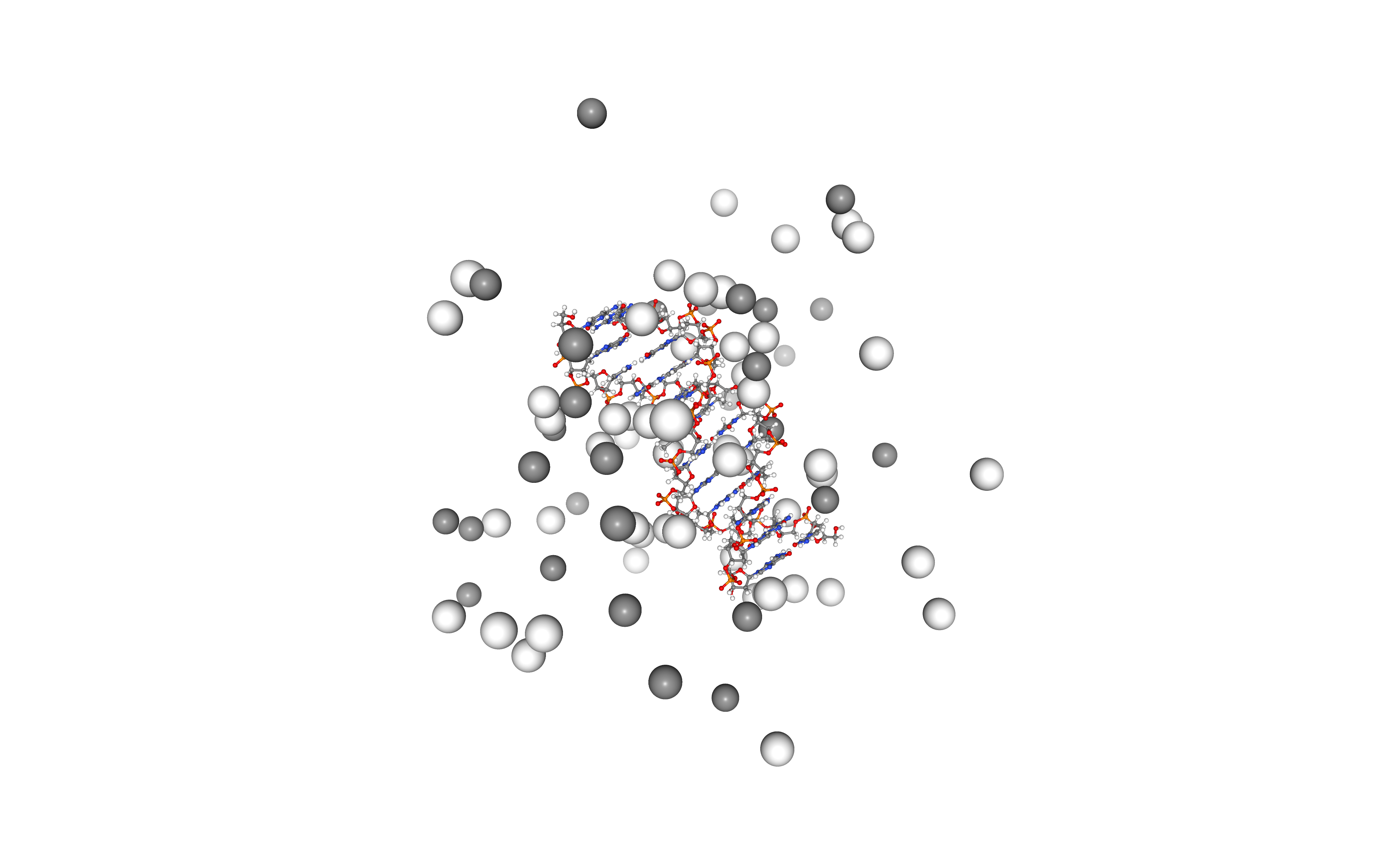
Neutralizing the system and adding an additional ionic concentration using the leap tool from the AMBER MD package.
Using Potassium (K+) and Chloride (Cl-) counterions and an additional ionic concentration of 150mM.
Building Blocks used:
- leap_add_ions from biobb_amber.leap.leap_add_ions
# Import module
from biobb_amber.leap.leap_add_ions import leap_add_ions

# Create prop dict and inputs/outputs
prop = {
    'forcefield': forcefield,
    'water_type': water_model,
    'ions_type' : ions_model,
    'box_type': 'truncated_octahedron',
    'ionic_concentration' : 100,  # 100 Mol/L
    'positive_ions_type' : "K+"
}

output_ions_pdb_path = 'structure.ions.pdb'
output_ions_top_path = 'structure.ions.parmtop'
output_ions_crd_path = 'structure.ions.crd'

# Create and launch bb
leap_add_ions(input_pdb_path=output_solv_pdb_path,
           output_pdb_path=output_ions_pdb_path,
           output_top_path=output_ions_top_path,
           output_crd_path=output_ions_crd_path,
           properties=prop)
# Show protein
view = nglview.show_structure_file(output_ions_pdb_path)
view.clear_representations()
view.add_representation(repr_type='ball+stick', selection='nucleic')
view.add_representation(repr_type='spacefill', selection='Na+')
view.add_representation(repr_type='spacefill', selection='K+')
view.add_representation(repr_type='spacefill', selection='Cl-')
view._remote_call('setSize', target='Widget', args=['','600px'])
view
Randomize ions
Randomly swap the positions of solvent and ions using the cpptraj tool from the AMBER MD package.
Building Blocks used:
- cpptraj_randomize_ions from biobb_amber.cpptraj.cpptraj_randomize_ions
# Import module
from biobb_amber.cpptraj.cpptraj_randomize_ions import cpptraj_randomize_ions

# Create prop dict and inputs/outputs
prop = {
    "distance" : 6.0,
    "overlap" : 4.0
}
output_cpptraj_crd_path = 'structure.randIons.crd'
output_cpptraj_pdb_path = 'structure.randIons.pdb'

# Create and launch bb
cpptraj_randomize_ions(
            input_top_path=output_ions_top_path,
            input_crd_path=output_ions_crd_path,
            output_pdb_path=output_cpptraj_pdb_path,
            output_crd_path=output_cpptraj_crd_path,
            properties=prop)
# Show protein
view = nglview.show_structure_file(output_cpptraj_pdb_path)
view.clear_representations()
view.add_representation(repr_type='ball+stick', selection='nucleic')
view.add_representation(repr_type='spacefill', selection='K+')
view.add_representation(repr_type='spacefill', selection='Cl-')
view._remote_call('setSize', target='Widget', args=['','600px'])
view
Generate Topology with Hydrogen Mass Partitioning (4fs)
Modifying the DNA topology from the modelled structure, tripling the mass of all hydrogens on the system and scaling down the mass of all other atoms using the parmed tool from the AMBER MD package.
Building Blocks used:
- parmed_hmassrepartition from biobb_amber.parmed.parmed_hmassrepartition
# Import module
from biobb_amber.parmed.parmed_hmassrepartition import parmed_hmassrepartition

# Create prop dict and inputs/outputs
dna_leap_top_4fs_path = 'structure.leap.4fs.top'

# Create and launch bb
parmed_hmassrepartition(
    input_top_path=output_ions_top_path,
    output_top_path=dna_leap_top_4fs_path
)
Standard Equilibration for explicit solvent
With the DNA + solvent + counterions system ready, the next step in the MD setup is the system equilibration. In this step, atoms of the macromolecules and of the surrounding solvent undergo a relaxation that usually lasts for tens or hundreds of picoseconds before the system reaches a stationary state (see Amber tutorials).
Many different equilibration protocols exist. The protocol included in this workflow was prepared, tested and compared with different conditions and DNA sequences by the ABC consortium, and finally chosen as the standard protocol for the 2021 ABCix run. It is based on the Daniel R. Roe and Bernard R. Brooks work (A protocol for preparing explicitly solvated systems for stable molecular dynamics simulations) and comprises 10 different stages:
- Equilibration Step 1 -- System Energetic Minimization, 5 Kcal/mol heavy atoms restraints (1000 cycles)
- Equilibration Step 2 -- NVT Equilibration, 5 Kcal/mol heavy atoms restraints, timestep 1fs (15ps)
- Equilibration Step 3 -- System Energetic Minimization, 2 Kcal/mol heavy atoms restraints (1000 cycles)
- Equilibration Step 4 -- System Energetic Minimization, 0.1 Kcal/mol heavy atoms restraints (1000 cycles)
- Equilibration Step 5 -- System Energetic Minimization (1000 cycles)
- Equilibration Step 6 -- NPT Equilibration, 1 Kcal/mol heavy atoms restraints, timestep 1fs (5ps)
- Equilibration Step 7 -- NPT Equilibration, 0.5 Kcal/mol heavy atoms restraints, timestep 1fs (5ps)
- Equilibration Step 8 -- NPT Equilibration, 0.5 Kcal/mol backbone atoms restraints, timestep 1fs (10ps)
- Equilibration Step 9 -- NPT Equilibration, timestep 2fs (10ps)
- Equilibration Step 10 -- NPT Equilibration, timestep 2fs, long simulation (1ns)
Equilibration Step 1: System energetic minimization
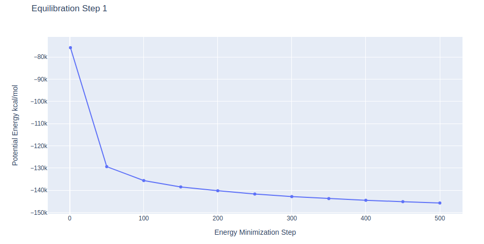
Energetically minimize the DNA structure (in solvent) using the sander tool from the AMBER MD package. Relaxing solvent molecules around the DNA structure.
AMBER MD configuration file used (step1.in) includes the following simulation parameters:
- imin = 1; Run minimization
- ntmin = 2; Steepest Descent minimization method
- maxcyc = 1000; Number of minimization steps
- ncyc = 10; Switch from steepest descent to conjugate gradient after 10 cycles (if ntmin = 1)
- ntwx = 500; Coordinates will be written to the output trajectory file every 500 steps
- ioutfm = 1; Write trajectory in netcdf format
- ntxo = 2; Write restart in netcdf format
- ntpr = 50; Write energy information to files 'mdout' and 'mdinfo' every 50 steps
- ntwr = 500; Write information to restart file every 500 steps
- ntc = 1; Turn off SHAKE for constraining length of bonds involving Hydrogen atoms
- ntf = 1; Force evaluation: complete interactions are calculated
- ntb = 1; Constant Volume Periodic Boundary Conditions (PBC)
- cut = 8.0; Cutoff for non bonded interactions in Angstroms
- ntr = 1; Turn on positional restraints
- restraintmask = :1-40&!@H=; Restraints on DNA atoms only
- restraint_wt = 5.0; Restraint force constant
Minimization step applying restraints on the DNA heavy atoms with a force constant of 5 Kcal/mol.Å2
Building Blocks used:
- sander_mdrun from biobb_amber.sander.sander_mdrun
- process_minout from biobb_amber.process.process_minout
# Import module
from biobb_amber.sander.sander_mdrun import sander_mdrun

# Create prop dict and inputs/outputs
prop = {
    "mdin" : {
        'maxcyc' : 500,  # Overwrite number of minimization steps if needed
        'restraintmask' : '\":DA,DC,DG,DT,D=3,D=5&!@H=\"' # Overwrite DNA heavy atoms mask to make it more generic
    },
#    "sander_path" : "sander.MPI",  # Change sander binary to parallel (MPI) execution (not included in AmberTools)
#    "mpi_bin" : "mpirun",          # MPI runner
#    "mpi_np" : 16                  # Number of cores to use in the MPI parallel calculation
}
output_eq1_traj_path = 'sander.eq1.nc'
output_eq1_rst_path = 'sander.eq1.ncrst'
output_eq1_log_path = 'sander.eq1.log'
output_eq1_mdinfo_path = 'sander.eq1.mdinfo'

# Create and launch bb
sander_mdrun(
            input_top_path=dna_leap_top_4fs_path,
            input_mdin_path="ABCix_config_files/step1.in",
            input_crd_path=output_cpptraj_crd_path,
            input_ref_path=output_cpptraj_crd_path,
            output_traj_path=output_eq1_traj_path,
            output_rst_path=output_eq1_rst_path,
            output_mdinfo_path=output_eq1_mdinfo_path,
            output_log_path=output_eq1_log_path,
            properties=prop)
# Import module
from biobb_amber.process.process_minout import process_minout

# Create prop dict and inputs/outputs
prop = {
    "terms" : ['ENERGY'],
    "remove_tmp": True
}
output_dat_eq1_path = 'sander.eq1.energy.dat'

# Create and launch bb
process_minout(input_log_path=output_eq1_log_path,
            output_dat_path=output_dat_eq1_path,
            properties=prop)
import plotly.graph_objs as go

with open(output_dat_eq1_path, 'r') as energy_file:
    x, y = zip(*[
        (float(line.split()[0]), float(line.split()[1]))
        for line in energy_file
        if not line.startswith(("#", "@"))
        if float(line.split()[1]) < 1000
    ])

# Create a scatter plot
fig = go.Figure(data=go.Scatter(x=x, y=y, mode='lines'))

# Update layout
fig.update_layout(title="Equilibration Step 1",
                  xaxis_title="Energy Minimization Step",
                  yaxis_title="Potential Energy kcal/mol",
                  height=600)

# Show the figure (renderer changes for colab and jupyter)
rend = 'colab' if 'google.colab' in sys.modules else ''
fig.show(renderer=rend)
Equilibration Step 2: NVT equilibration
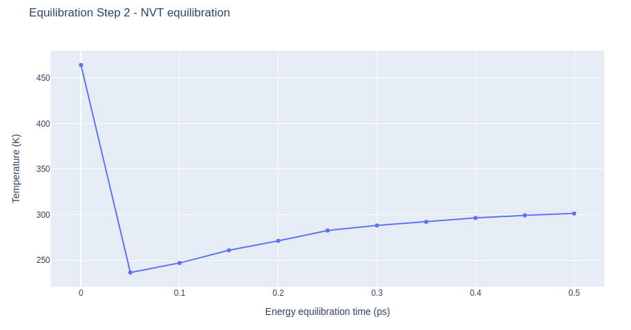
Equilibrate the system in NVT ensemble (constant number of particles -N-, Volume -V-, and Temperature -T-), using the sander tool from the AMBER MD package. Taking the system to the desired temperature.
AMBER MD configuration file used (step2.in) includes the following simulation parameters:
- imin = 0; Run MD (no minimization)
- nstlim = 15000; Number of MD steps
- dt = 0.001; Time step (in ps)
- ntx = 1; Only read initial coordinates from input files
- irest = 0; Do not restart a simulation, start a new one
- ig = -1; Seed for the pseudo-random number generator
- ntwx = 500; Coordinates will be written to the output trajectory file every 500 steps
- ntwv = -1; Velocities will be written to output trajectory file, making it a combined coordinate/velocity trajectory file, at the interval defined by ntwx
- ioutfm = 1; Write trajectory in netcdf format
- ntxo = 2; Write restart in netcdf format
- ntpr = 50; Write energy information to files 'mdout' and 'mdinfo' every 50 steps
- ntwr = 500; Write information to restart file every 500 steps
- iwrap = 0; Not wrapping coordinates into primary box
- nscm = 0; Not removing translational and rotational center-of-mass motions
- ntc = 2; Turn on SHAKE for constraining length of bonds involving Hydrogen atoms
- ntf = 2; Force evaluation: Bond interactions involving H omitted (SHAKE)
- ntb = 1; Constant Volume Periodic Boundary Conditions (PBC)
- cut = 8.0; Cutoff for non bonded interactions in Angstroms
- ntt = 3; Constant temperature using Langevin dynamics
- gamma_ln = 5; Collision frequency for Langevin dynamics (in 1/ps)
- temp0 = 310.0; Final temperature (310 K)
- tempi = 310.0; Initial temperature (310 K)
- ntr = 1; Turn on positional restraints
- restraintmask = :1-40&!@H=; Restraints on DNA atoms only
- restraint_wt = 5.0; Restraint force constant
NVT equilibration step applying restraints on the DNA heavy atoms with a force constant of 5 Kcal/mol.Å2
Building Blocks used:
- sander_mdrun from biobb_amber.sander.sander_mdrun
- process_mdout from biobb_amber.process.process_mdout
# Import module
from biobb_amber.sander.sander_mdrun import sander_mdrun

# Create prop dict and inputs/outputs
prop = {
    "mdin" : {
        'nstlim' : 500,  # Overwrite number of MD steps if needed
        'restraintmask' : '\":DA,DC,DG,DT,D=3,D=5&!@H=\"' # Overwrite DNA heavy atoms mask to make it more generic
    },
#    "sander_path" : "sander.MPI",  # Change sander binary to parallel (MPI) execution (not included in AmberTools)
#    "mpi_bin" : "mpirun",          # MPI runner
#    "mpi_np" : 16                  # Number of cores to use in the MPI parallel calculation
}
output_eq2_traj_path = 'sander.eq2.nc'
output_eq2_rst_path = 'sander.eq2.ncrst'
output_eq2_log_path = 'sander.eq2.log'
output_eq2_mdinfo_path = 'sander.eq2.mdinfo'

# Create and launch bb
sander_mdrun(input_top_path=dna_leap_top_4fs_path,
            input_mdin_path="ABCix_config_files/step2.in",
            input_crd_path=output_eq1_rst_path,
            input_ref_path=output_eq1_rst_path,
            output_traj_path=output_eq2_traj_path,
            output_rst_path=output_eq2_rst_path,
            output_log_path=output_eq2_log_path,
            output_mdinfo_path=output_eq2_mdinfo_path,
            properties=prop)
# Import module
from biobb_amber.process.process_mdout import process_mdout

# Create prop dict and inputs/outputs
prop = {
    "terms" : ['TEMP']
}
output_dat_eq2_path = 'sander.eq2.energy.dat'

# Create and launch bb
process_mdout(input_log_path=output_eq2_log_path,
            output_dat_path=output_dat_eq2_path,
            properties=prop)
import plotly.graph_objs as go

with open(output_dat_eq2_path, 'r') as energy_file:
    x, y = zip(*[
        (float(line.split()[0]), float(line.split()[1]))
        for line in energy_file
        if not line.startswith(("#", "@"))
        if float(line.split()[1]) < 1000
    ])

# Create a scatter plot
fig = go.Figure(data=go.Scatter(x=x, y=y, mode='lines'))

# Update layout
fig.update_layout(title="Equilibration Step 2 - NVT equilibration",
                  xaxis_title="Energy equilibration time (ps)",
                  yaxis_title="Temperature (K)",
                  height=600)

# Show the figure (renderer changes for colab and jupyter)
rend = 'colab' if 'google.colab' in sys.modules else ''
fig.show(renderer=rend)
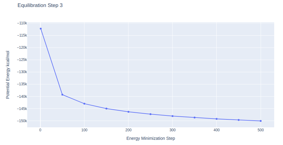
Equilibration Step 3: System energetic minimization
Energetically minimize the DNA structure (in solvent) using the sander tool from the AMBER MD package. Relaxing system with soft restraints on the DNA structure.
AMBER MD configuration file used (step3.in) includes the following simulation parameters:
- imin = 1; Run minimization
- ntmin = 2; Steepest Descent minimization method
- maxcyc = 1000; Number of minimization steps
- ncyc = 10; Switch from steepest descent to conjugate gradient after 10 cycles (if ntmin = 1)
- ntwx = 500; Coordinates will be written to the output trajectory file every 500 steps
- ioutfm = 1; Write trajectory in netcdf format
- ntxo = 2; Write restart in netcdf format
- ntpr = 50; Write energy information to files 'mdout' and 'mdinfo' every 50 steps
- ntwr = 500; Write information to restart file every 500 steps
- ntc = 1; Turn off SHAKE for constraining length of bonds involving Hydrogen atoms
- ntf = 1; Force evaluation: complete interactions are calculated
- ntb = 1; Constant Volume Periodic Boundary Conditions (PBC)
- cut = 8.0; Cutoff for non bonded interactions in Angstroms
- ntr = 1; Turn on positional restraints
- restraintmask = :1-40&!@H=; Restraints on DNA atoms only
- restraint_wt = 2.0; Restraint force constant
Further minimization step lowering the restraints on the DNA heavy atoms to 2 Kcal/mol.Å2 force constant.
Building Blocks used:
- sander_mdrun from biobb_amber.sander.sander_mdrun
- process_minout from biobb_amber.process.process_minout
# Import module
from biobb_amber.sander.sander_mdrun import sander_mdrun

# Create prop dict and inputs/outputs
prop = {
    "mdin" : {
        'maxcyc' : 500,  # Overwrite number of minimization steps if needed
        'restraintmask' : '\":DA,DC,DG,DT,D=3,D=5&!@H=\"' # Overwrite DNA heavy atoms mask to make it more generic
    },
#    "sander_path" : "sander.MPI",  # Change sander binary to parallel (MPI) execution (not included in AmberTools)
#    "mpi_bin" : "mpirun",          # MPI runner
#    "mpi_np" : 16                  # Number of cores to use in the MPI parallel calculation
}
output_eq3_traj_path = 'sander.eq3.nc'
output_eq3_rst_path = 'sander.eq3.ncrst'
output_eq3_log_path = 'sander.eq3.log'
output_eq3_mdinfo_path = 'sander.eq3.mdinfo'

# Create and launch bb
sander_mdrun(input_top_path=dna_leap_top_4fs_path,
            input_mdin_path="ABCix_config_files/step3.in",
            input_crd_path=output_eq2_rst_path,
            input_ref_path=output_eq2_rst_path,
            output_traj_path=output_eq3_traj_path,
            output_rst_path=output_eq3_rst_path,
            output_log_path=output_eq3_log_path,
            output_mdinfo_path=output_eq3_mdinfo_path,
            properties=prop)
# Import module
from biobb_amber.process.process_minout import process_minout

# Create prop dict and inputs/outputs
prop = {
    "terms" : ['ENERGY']
}
output_dat_eq3_path = 'sander.eq3.energy.dat'

# Create and launch bb
process_minout(input_log_path=output_eq3_log_path,
            output_dat_path=output_dat_eq3_path,
            properties=prop)
import plotly.graph_objs as go

with open(output_dat_eq3_path, 'r') as energy_file:
    x, y = zip(*[
        (float(line.split()[0]), float(line.split()[1]))
        for line in energy_file
        if not line.startswith(("#", "@"))
        if float(line.split()[1]) < 1000
    ])

# Create a scatter plot
fig = go.Figure(data=go.Scatter(x=x, y=y, mode='lines'))

# Update layout
fig.update_layout(title="Equilibration Step 3",
                  xaxis_title="Energy Minimization Step",
                  yaxis_title="Potential Energy kcal/mol",
                  height=600)

# Show the figure (renderer changes for colab and jupyter)
rend = 'colab' if 'google.colab' in sys.modules else ''
fig.show(renderer=rend)
Equilibration Step 4: System energetic minimization
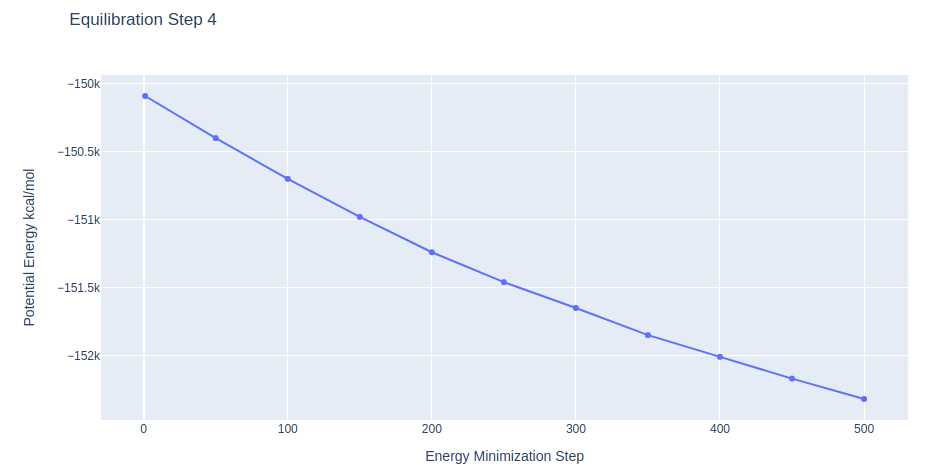
Energetically minimize the DNA structure (in solvent) using the sander tool from the AMBER MD package. Relaxing system with minimum restraints on the DNA structure.
AMBER MD configuration file used (step4.in) includes the following simulation parameters:
- imin = 1; Run minimization
- ntmin = 2; Steepest Descent minimization method
- maxcyc = 1000; Number of minimization steps
- ncyc = 10; Switch from steepest descent to conjugate gradient after 10 cycles (if ntmin = 1)
- ntwx = 500; Coordinates will be written to the output trajectory file every 500 steps
- ioutfm = 1; Write trajectory in netcdf format
- ntxo = 2; Write restart in netcdf format
- ntpr = 50; Write energy information to files 'mdout' and 'mdinfo' every 50 steps
- ntwr = 500; Write information to restart file every 500 steps
- ntc = 1; Turn off SHAKE for constraining length of bonds involving Hydrogen atoms
- ntf = 1; Force evaluation: complete interactions are calculated
- ntb = 1; Constant Volume Periodic Boundary Conditions (PBC)
- cut = 8.0; Cutoff for non bonded interactions in Angstroms
- ntr = 1; Turn on positional restraints
- restraintmask = :1-40&!@H=; Restraints on DNA atoms only
- restraint_wt = 0.1; Restraint force constant
Further minimization step lowering the restraints on the DNA heavy atoms to 0.1 Kcal/mol.Å2 force constant.
Building Blocks used:
- sander_mdrun from biobb_amber.sander.sander_mdrun
- process_minout from biobb_amber.process.process_minout
# Import module
from biobb_amber.sander.sander_mdrun import sander_mdrun

# Create prop dict and inputs/outputs
prop = {
    "mdin" : {
        'maxcyc' : 500,  # Overwrite number of minimization steps if needed
        'restraintmask' : '\":DA,DC,DG,DT,D=3,D=5&!@H=\"' # Overwrite DNA heavy atoms mask to make it more generic
    },
#    "sander_path" : "sander.MPI",  # Change sander binary to parallel (MPI) execution (not included in AmberTools)
#    "mpi_bin" : "mpirun",          # MPI runner
#    "mpi_np" : 16                  # Number of cores to use in the MPI parallel calculation
}
output_eq4_traj_path = 'sander.eq4.nc'
output_eq4_rst_path = 'sander.eq4.ncrst'
output_eq4_log_path = 'sander.eq4.log'
output_eq4_mdinfo_path = 'sander.eq4.mdinfo'

# Create and launch bb
sander_mdrun(input_top_path=dna_leap_top_4fs_path,
            input_mdin_path="ABCix_config_files/step4.in",
            input_crd_path=output_eq3_rst_path,
            input_ref_path=output_eq3_rst_path,
            output_traj_path=output_eq4_traj_path,
            output_rst_path=output_eq4_rst_path,
            output_log_path=output_eq4_log_path,
            output_mdinfo_path=output_eq4_mdinfo_path,
            properties=prop)
# Import module
from biobb_amber.process.process_minout import process_minout

# Create prop dict and inputs/outputs
prop = {
    "terms" : ['ENERGY']
}
output_dat_eq4_path = 'sander.eq4.energy.dat'

# Create and launch bb
process_minout(input_log_path=output_eq4_log_path,
            output_dat_path=output_dat_eq4_path,
            properties=prop)
import plotly.graph_objs as go

with open(output_dat_eq4_path, 'r') as energy_file:
    x, y = zip(*[
        (float(line.split()[0]), float(line.split()[1]))
        for line in energy_file
        if not line.startswith(("#", "@"))
        if float(line.split()[1]) < 1000
    ])

# Create a scatter plot
fig = go.Figure(data=go.Scatter(x=x, y=y, mode='lines'))

# Update layout
fig.update_layout(title="Equilibration Step 4",
                  xaxis_title="Energy Minimization Step",
                  yaxis_title="Potential Energy kcal/mol",
                  height=600)

# Show the figure (renderer changes for colab and jupyter)
rend = 'colab' if 'google.colab' in sys.modules else ''
fig.show(renderer=rend)
Equilibration Step 5: System energetic minimization
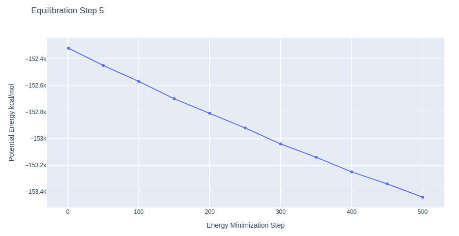
Energetically minimize the DNA structure (in solvent) using the sander tool from the AMBER MD package. Relaxing system without restraints on the DNA structure.
AMBER MD configuration file used (step5.in) includes the following simulation parameters:
- imin = 1; Run minimization
- ntmin = 2; Steepest Descent minimization method
- maxcyc = 1000; Number of minimization steps
- ncyc = 10; Switch from steepest descent to conjugate gradient after 10 cycles (if ntmin = 1)
- ntwx = 500; Coordinates will be written to the output trajectory file every 500 steps
- ioutfm = 1; Write trajectory in netcdf format
- ntxo = 2; Write restart in netcdf format
- ntpr = 50; Write energy information to files 'mdout' and 'mdinfo' every 50 steps
- ntwr = 500; Write information to restart file every 500 steps
- ntc = 1; Turn off SHAKE for constraining length of bonds involving Hydrogen atoms
- ntf = 1; Force evaluation: complete interactions are calculated
- ntb = 1; Constant Volume Periodic Boundary Conditions (PBC)
- cut = 8.0; Cutoff for non bonded interactions in Angstroms
- ntr = 0; Turn off positional restraints
Further minimization step, with all position restraints on the DNA heavy atoms released.
Building Blocks used:
- sander_mdrun from biobb_amber.sander.sander_mdrun
- process_minout from biobb_amber.process.process_minout
# Import module
from biobb_amber.sander.sander_mdrun import sander_mdrun

# Create prop dict and inputs/outputs
prop = {
    "mdin" : {
        'maxcyc' : 500  # Overwrite number of minimization steps if needed
    },
#    "sander_path" : "sander.MPI",  # Change sander binary to parallel (MPI) execution (not included in AmberTools)
#    "mpi_bin" : "mpirun",          # MPI runner
#    "mpi_np" : 16                  # Number of cores to use in the MPI parallel calculation
}
output_eq5_traj_path = 'sander.eq5.nc'
output_eq5_rst_path = 'sander.eq5.ncrst'
output_eq5_log_path = 'sander.eq5.log'
output_eq5_mdinfo_path = 'sander.eq5.mdinfo'

# Create and launch bb
sander_mdrun(input_top_path=dna_leap_top_4fs_path,
            input_mdin_path="ABCix_config_files/step5.in",
            input_crd_path=output_eq4_rst_path,
            input_ref_path=output_eq4_rst_path,
            output_traj_path=output_eq5_traj_path,
            output_rst_path=output_eq5_rst_path,
            output_log_path=output_eq5_log_path,
            output_mdinfo_path=output_eq5_mdinfo_path,
            properties=prop)
# Import module
from biobb_amber.process.process_minout import process_minout

# Create prop dict and inputs/outputs
prop = {
    "terms" : ['ENERGY']
}
output_dat_eq5_path = 'sander.eq5.energy.dat'

# Create and launch bb
process_minout(input_log_path=output_eq5_log_path,
            output_dat_path=output_dat_eq5_path,
            properties=prop)
import plotly.graph_objs as go

with open(output_dat_eq5_path, 'r') as energy_file:
    x, y = zip(*[
        (float(line.split()[0]), float(line.split()[1]))
        for line in energy_file
        if not line.startswith(("#", "@"))
        if float(line.split()[1]) < 1000
    ])

# Create a scatter plot
fig = go.Figure(data=go.Scatter(x=x, y=y, mode='lines'))

# Update layout
fig.update_layout(title="Equilibration Step 5",
                  xaxis_title="Energy Minimization Step",
                  yaxis_title="Potential Energy kcal/mol",
                  height=600)

# Show the figure (renderer changes for colab and jupyter)
rend = 'colab' if 'google.colab' in sys.modules else ''
fig.show(renderer=rend)
Equilibration Step 6: NPT equilibration
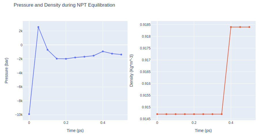
Equilibrate the system in NPT ensemble (constant number of particles -N-, Pressure -P-, and Temperature -T-), using the sander tool from the AMBER MD package.
AMBER MD configuration file used (step6.in) includes the following simulation parameters:
- imin = 0; Run MD (no minimization)
- nstlim = 5000; Number of MD steps
- dt = 0.001; Time step (in ps)
- ntx = 1; Only read initial coordinates from input files
- irest = 0; Do not restart a simulation, start a new one
- ig = -1; Seed for the pseudo-random number generator
- ntwx = 500; Coordinates will be written to the output trajectory file every 500 steps
- ntwv = -1; Velocities will be written to output trajectory file, making it a combined coordinate/velocity trajectory file, at the interval defined by ntwx
- ioutfm = 1; Write trajectory in netcdf format
- ntxo = 2; Write restart in netcdf format
- ntpr = 50; Write energy information to files 'mdout' and 'mdinfo' every 50 steps
- ntwr = 500; Write information to restart file every 500 steps
- iwrap = 0; Not wrapping coordinates into primary box
- nscm = 0; Not removing translational and rotational center-of-mass motions
- ntc = 2; Turn on SHAKE for constraining length of bonds involving Hydrogen atoms
- ntf = 2; Force evaluation: Bond interactions involving H omitted (SHAKE)
- ntb = 2; Constant Pressure Periodic Boundary Conditions (PBC)
- cut = 8.0; Cutoff for non bonded interactions in Angstroms
- ntt = 3; Constant temperature using Langevin dynamics
- gamma_ln = 5; Collision frequency for Langevin dynamics (in 1/ps)
- temp0 = 310.0; Final temperature (310 K)
- tempi = 310.0; Initial temperature (310 K)
- ntp = 1; Constant pressure dynamics: md with isotropic position scaling
- barostat = 2; Monte Carlo Barostat
- pres0 = 1.0; Reference pressure at which the system is maintained
- ntr = 1; Turn on positional restraints
- restraintmask = :1-40&!@H=; Restraints on DNA atoms only
- restraint_wt = 1.0; Restraint force constant
NPT equilibration step applying restraints on the DNA heavy atoms with a force constant of 1 Kcal/mol.Å2
Building Blocks used:
- sander_mdrun from biobb_amber.sander.sander_mdrun
- process_mdout from biobb_amber.process.process_mdout
# Import module
from biobb_amber.sander.sander_mdrun import sander_mdrun

# Create prop dict and inputs/outputs
prop = {
    "mdin" : {
        'nstlim' : 500,  # Overwrite number of MD steps if needed
        'restraintmask' : '\":DA,DC,DG,DT,D=3,D=5&!@H=\"' # Overwrite DNA heavy atoms mask to make it more generic
    },
#    "sander_path" : "sander.MPI",  # Change sander binary to parallel (MPI) execution (not included in AmberTools)
#    "mpi_bin" : "mpirun",          # MPI runner
#    "mpi_np" : 16                  # Number of cores to use in the MPI parallel calculation
}
output_eq6_traj_path = 'sander.eq6.nc'
output_eq6_rst_path = 'sander.eq6.ncrst'
output_eq6_log_path = 'sander.eq6.log'
output_eq6_mdinfo_path = 'sander.eq6.mdinfo'

# Create and launch bb
sander_mdrun(input_top_path=dna_leap_top_4fs_path,
            input_mdin_path="ABCix_config_files/step6.in",
            input_crd_path=output_eq5_rst_path,
            input_ref_path=output_eq5_rst_path,
            output_traj_path=output_eq6_traj_path,
            output_rst_path=output_eq6_rst_path,
            output_log_path=output_eq6_log_path,
            output_mdinfo_path=output_eq6_mdinfo_path,
            properties=prop)
# Import module
from biobb_amber.process.process_mdout import process_mdout

# Create prop dict and inputs/outputs
prop = {
    "terms" : ['PRES','DENSITY']
}
output_dat_eq6_path = 'sander.eq6.pressure_and_density.dat'

# Create and launch bb
process_mdout(input_log_path=output_eq6_log_path,
            output_dat_path=output_dat_eq6_path,
            properties=prop)
# Read pressure and density data from file
import plotly.graph_objs as go
from plotly import subplots

# Read pressure and density data from file
with open(output_dat_eq6_path, 'r') as pd_file:
    x, y, z = zip(*[
        (float(line.split()[0]), float(line.split()[1]), float(line.split()[2]))
        for line in pd_file
        if not line.startswith(("#", "@"))
    ])

# Create a scatter plot
trace1 = go.Scatter(
    x=x,y=y
)
trace2 = go.Scatter(
    x=x,y=z
)

fig = subplots.make_subplots(rows=1, cols=2, print_grid=False)

fig.append_trace(trace1, 1, 1)
fig.append_trace(trace2, 1, 2)

fig['layout']['xaxis1'].update(title='Time (ps)')
fig['layout']['xaxis2'].update(title='Time (ps)')
fig['layout']['yaxis1'].update(title='Pressure (bar)')
fig['layout']['yaxis2'].update(title='Density (Kg*m^-3)')

fig['layout'].update(title='Pressure and Density during NPT Equilibration')
fig['layout'].update(showlegend=False)
fig['layout'].update(height=500)

# Show the figure (renderer changes for colab and jupyter)
rend = 'colab' if 'google.colab' in sys.modules else ''
fig.show(renderer=rend)
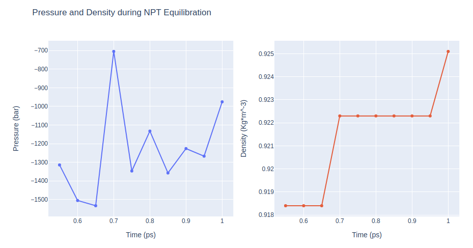
Equilibration Step 7: NPT equilibration
Equilibrate the system in NPT ensemble (constant number of particles -N-, Pressure -P-, and Temperature -T-), using the sander tool from the AMBER MD package. Lowering restraints force constant.
AMBER MD configuration file used (step7.in) includes the following simulation parameters:
- imin = 0; Run MD (no minimization)
- nstlim = 5000; Number of MD steps
- dt = 0.001; Time step (in ps)
- ntx = 5; Read initial coordinates and velocities from restart file
- irest = 1; Restart previous simulation from restart file
- ig = -1; Seed for the pseudo-random number generator
- ntwx = 500; Coordinates will be written to the output trajectory file every 500 steps
- ntwv = -1; Velocities will be written to output trajectory file, making it a combined coordinate/velocity trajectory file, at the interval defined by ntwx
- ioutfm = 1; Write trajectory in netcdf format
- ntxo = 2; Write restart in netcdf format
- ntpr = 50; Write energy information to files 'mdout' and 'mdinfo' every 50 steps
- ntwr = 500; Write information to restart file every 500 steps
- iwrap = 0; Not wrapping coordinates into primary box
- nscm = 0; Not removing translational and rotational center-of-mass motions
- ntc = 2; Turn on SHAKE for constraining length of bonds involving Hydrogen atoms
- ntf = 2; Force evaluation: Bond interactions involving H omitted (SHAKE)
- ntb = 2; Constant Pressure Periodic Boundary Conditions (PBC)
- cut = 8.0; Cutoff for non bonded interactions in Angstroms
- ntt = 3; Constant temperature using Langevin dynamics
- gamma_ln = 5; Collision frequency for Langevin dynamics (in 1/ps)
- temp0 = 310.0; Final temperature (310 K)
- tempi = 310.0; Initial temperature (310 K)
- ntp = 1; Constant pressure dynamics: md with isotropic position scaling
- barostat = 2; Monte Carlo Barostat
- pres0 = 1.0; Reference pressure at which the system is maintained
- ntr = 1; Turn on positional restraints
- restraintmask = :1-40&!@H=; Restraints on DNA atoms only
- restraint_wt = 0.5; Restraint force constant
NPT equilibration step applying restraints on the DNA heavy atoms with a force constant of 0.5 Kcal/mol.Å2.
Restarting from previous equilibration step.
Building Blocks used:
- sander_mdrun from biobb_amber.sander.sander_mdrun
- process_mdout from biobb_amber.process.process_mdout
# Import module
from biobb_amber.sander.sander_mdrun import sander_mdrun

# Create prop dict and inputs/outputs
prop = {
    "mdin" : {
        'nstlim' : 500,  # Overwrite number of MD steps if needed
        'restraintmask' : '\":DA,DC,DG,DT,D=3,D=5&!@H=\"' # Overwrite DNA heavy atoms mask to make it more generic
    },
#    "sander_path" : "sander.MPI",  # Change sander binary to parallel (MPI) execution (not included in AmberTools)
#    "mpi_bin" : "mpirun",          # MPI runner
#    "mpi_np" : 16                  # Number of cores to use in the MPI parallel calculation
}
output_eq7_traj_path = 'sander.eq7.nc'
output_eq7_rst_path = 'sander.eq7.ncrst'
output_eq7_log_path = 'sander.eq7.log'
output_eq7_mdinfo_path = 'sander.eq7.mdinfo'

# Create and launch bb
sander_mdrun(input_top_path=dna_leap_top_4fs_path,
            input_mdin_path="ABCix_config_files/step7.in",
            input_crd_path=output_eq6_rst_path,
            input_ref_path=output_eq6_rst_path,
            output_traj_path=output_eq7_traj_path,
            output_rst_path=output_eq7_rst_path,
            output_log_path=output_eq7_log_path,
            output_mdinfo_path=output_eq7_mdinfo_path,
            properties=prop)
# Import module
from biobb_amber.process.process_mdout import process_mdout

# Create prop dict and inputs/outputs
prop = {
    "terms" : ['PRES','DENSITY']
}
output_dat_eq7_path = 'sander.eq7.pressure_and_density.dat'

# Create and launch bb
process_mdout(input_log_path=output_eq7_log_path,
            output_dat_path=output_dat_eq7_path,
            properties=prop)
# Read pressure and density data from file
import plotly.graph_objs as go
from plotly import subplots

# Read pressure and density data from file
with open(output_dat_eq7_path, 'r') as pd_file:
    x, y, z = zip(*[
        (float(line.split()[0]), float(line.split()[1]), float(line.split()[2]))
        for line in pd_file
        if not line.startswith(("#", "@"))
    ])

# Create a scatter plot
trace1 = go.Scatter(
    x=x,y=y
)
trace2 = go.Scatter(
    x=x,y=z
)

fig = subplots.make_subplots(rows=1, cols=2, print_grid=False)

fig.append_trace(trace1, 1, 1)
fig.append_trace(trace2, 1, 2)

fig['layout']['xaxis1'].update(title='Time (ps)')
fig['layout']['xaxis2'].update(title='Time (ps)')
fig['layout']['yaxis1'].update(title='Pressure (bar)')
fig['layout']['yaxis2'].update(title='Density (Kg*m^-3)')

fig['layout'].update(title='Pressure and Density during NPT Equilibration')
fig['layout'].update(showlegend=False)
fig['layout'].update(height=500)

# Show the figure (renderer changes for colab and jupyter)
rend = 'colab' if 'google.colab' in sys.modules else ''
fig.show(renderer=rend)
Equilibration Step 8: NPT equilibration
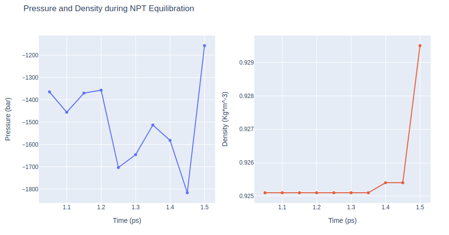
Equilibrate the system in NPT ensemble (constant number of particles -N-, Pressure -P-, and Temperature -T-), using the sander tool from the AMBER MD package. Releasing position restraints from the atoms of the DNA bases (keeping only backbone atoms restrained).
AMBER MD configuration file used (step8.in) includes the following simulation parameters:
- imin = 0; Run MD (no minimization)
- nstlim = 10000; Number of MD steps
- dt = 0.001; Time step (in ps)
- ntx = 5; Read initial coordinates and velocities from restart file
- irest = 1; Restart previous simulation from restart file
- ig = -1; Seed for the pseudo-random number generator
- ntwx = 500; Coordinates will be written to the output trajectory file every 500 steps
- ntwv = -1; Velocities will be written to output trajectory file, making it a combined coordinate/velocity trajectory file, at the interval defined by ntwx
- ioutfm = 1; Write trajectory in netcdf format
- ntxo = 2; Write restart in netcdf format
- ntpr = 50; Write energy information to files 'mdout' and 'mdinfo' every 50 steps
- ntwr = 500; Write information to restart file every 500 steps
- iwrap = 0; Not wrapping coordinates into primary box
- nscm = 0; Not removing translational and rotational center-of-mass motions
- ntc = 2; Turn on SHAKE for constraining length of bonds involving Hydrogen atoms
- ntf = 2; Force evaluation: Bond interactions involving H omitted (SHAKE)
- ntb = 2; Constant Pressure Periodic Boundary Conditions (PBC)
- cut = 8.0; Cutoff for non bonded interactions in Angstroms
- ntt = 3; Constant temperature using Langevin dynamics
- gamma_ln = 5; Collision frequency for Langevin dynamics (in 1/ps)
- temp0 = 310.0; Final temperature (310 K)
- tempi = 310.0; Initial temperature (310 K)
- ntp = 1; Constant pressure dynamics: md with isotropic position scaling
- barostat = 2; Monte Carlo Barostat
- pres0 = 1.0; Reference pressure at which the system is maintained
- ntr = 1; Turn on positional restraints
- restraintmask = :1-40@P,O5',C5',C4',C3',O3'; Restraints on DNA atoms only
- restraint_wt = 0.5; Restraint force constant
NPT equilibration step applying restraints on the DNA backbone atoms with a force constant of 0.5 Kcal/mol.Å2.
Restarting from previous equilibration step.
Building Blocks used:
- sander_mdrun from biobb_amber.sander.sander_mdrun
- process_mdout from biobb_amber.process.process_mdout
# Import module
from biobb_amber.sander.sander_mdrun import sander_mdrun

# Create prop dict and inputs/outputs
prop = {
    "mdin" : {
        'nstlim' : 500,  # Overwrite number of MD steps if needed
        'restraintmask' : '\":DA,DC,DG,DT,D=3,D=5&@P,O5\',C5\',C4\',C3\',O3\'\"' # Overwrite DNA heavy atoms mask to make it more generic
    },
#    "sander_path" : "sander.MPI",  # Change sander binary to parallel (MPI) execution (not included in AmberTools)
#    "mpi_bin" : "mpirun",          # MPI runner
#    "mpi_np" : 16                  # Number of cores to use in the MPI parallel calculation
}
output_eq8_traj_path = 'sander.eq8.nc'
output_eq8_rst_path = 'sander.eq8.ncrst'
output_eq8_log_path = 'sander.eq8.log'
output_eq8_mdinfo_path = 'sander.eq8.mdinfo'

# Create and launch bb
sander_mdrun(input_top_path=dna_leap_top_4fs_path,
            input_mdin_path="ABCix_config_files/step8.in",
            input_crd_path=output_eq7_rst_path,
            input_ref_path=output_eq7_rst_path,
            output_traj_path=output_eq8_traj_path,
            output_rst_path=output_eq8_rst_path,
            output_log_path=output_eq8_log_path,
            output_mdinfo_path=output_eq8_mdinfo_path,
            properties=prop)
# Import module
from biobb_amber.process.process_mdout import process_mdout

# Create prop dict and inputs/outputs
prop = {
    "terms" : ['PRES','DENSITY']
}
output_dat_eq8_path = 'sander.eq8.pressure_and_density.dat'

# Create and launch bb
process_mdout(input_log_path=output_eq8_log_path,
            output_dat_path=output_dat_eq8_path,
            properties=prop)
# Read pressure and density data from file
import plotly.graph_objs as go
from plotly import subplots

# Read pressure and density data from file
with open(output_dat_eq8_path, 'r') as pd_file:
    x, y, z = zip(*[
        (float(line.split()[0]), float(line.split()[1]), float(line.split()[2]))
        for line in pd_file
        if not line.startswith(("#", "@"))
    ])

# Create a scatter plot
trace1 = go.Scatter(
    x=x,y=y
)
trace2 = go.Scatter(
    x=x,y=z
)

fig = subplots.make_subplots(rows=1, cols=2, print_grid=False)

fig.append_trace(trace1, 1, 1)
fig.append_trace(trace2, 1, 2)

fig['layout']['xaxis1'].update(title='Time (ps)')
fig['layout']['xaxis2'].update(title='Time (ps)')
fig['layout']['yaxis1'].update(title='Pressure (bar)')
fig['layout']['yaxis2'].update(title='Density (Kg*m^-3)')

fig['layout'].update(title='Pressure and Density during NPT Equilibration')
fig['layout'].update(showlegend=False)
fig['layout'].update(height=500)

# Show the figure (renderer changes for colab and jupyter)
rend = 'colab' if 'google.colab' in sys.modules else ''
fig.show(renderer=rend)
Equilibration Step 9: NPT equilibration
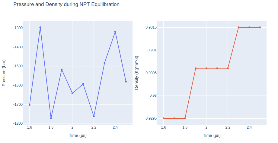
Equilibrate the system in NPT ensemble (constant number of particles -N-, Pressure -P-, and Temperature -T-), using the sander tool from the AMBER MD package. Releasing all position restraints.
AMBER MD configuration file used (step9.in) includes the following simulation parameters:
- imin = 0; Run MD (no minimization)
- nstlim = 5000; Number of MD steps
- dt = 0.002; Time step (in ps)
- ntx = 5; Read initial coordinates and velocities from restart file
- irest = 1; Restart previous simulation from restart file
- ig = -1; Seed for the pseudo-random number generator
- ntwx = 500; Coordinates will be written to the output trajectory file every 500 steps
- ntwv = -1; Velocities will be written to output trajectory file, making it a combined coordinate/velocity trajectory file, at the interval defined by ntwx
- ioutfm = 1; Write trajectory in netcdf format
- ntxo = 2; Write restart in netcdf format
- ntpr = 50; Write energy information to files 'mdout' and 'mdinfo' every 50 steps
- ntwr = 500; Write information to restart file every 500 steps
- iwrap = 0; Not wrapping coordinates into primary box
- nscm = 1000; Removing translational and rotational center-of-mass motions every 1000 steps
- ntc = 2; Turn on SHAKE for constraining length of bonds involving Hydrogen atoms
- ntf = 2; Force evaluation: Bond interactions involving H omitted (SHAKE)
- ntb = 2; Constant Pressure Periodic Boundary Conditions (PBC)
- cut = 8.0; Cutoff for non bonded interactions in Angstroms
- ntt = 3; Constant temperature using Langevin dynamics
- gamma_ln = 5; Collision frequency for Langevin dynamics (in 1/ps)
- temp0 = 310.0; Final temperature (310 K)
- tempi = 310.0; Initial temperature (310 K)
- ntp = 1; Constant pressure dynamics: md with isotropic position scaling
- barostat = 2; Monte Carlo Barostat
- pres0 = 1.0; Reference pressure at which the system is maintained
- ntr = 0; Turn off positional restraints
NPT equilibration step without any position restraints.
Removing translational and rotational center-of-mass motions. Timestep 2fs.
Restarting from previous equilibration step.
Building Blocks used:
- sander_mdrun from biobb_amber.sander.sander_mdrun
- process_mdout from biobb_amber.process.process_mdout
# Import module
from biobb_amber.sander.sander_mdrun import sander_mdrun

# Create prop dict and inputs/outputs
prop = {
    "mdin" : {
        'nstlim' : 500  # Overwrite number of MD steps if needed
    },
#    "sander_path" : "sander.MPI",  # Change sander binary to parallel (MPI) execution (not included in AmberTools)
#    "mpi_bin" : "mpirun",          # MPI runner
#    "mpi_np" : 16                  # Number of cores to use in the MPI parallel calculation
}
output_eq9_traj_path = 'sander.eq9.nc'
output_eq9_rst_path = 'sander.eq9.ncrst'
output_eq9_log_path = 'sander.eq9.log'
output_eq9_mdinfo_path = 'sander.eq9.mdinfo'

# Create and launch bb
sander_mdrun(input_top_path=dna_leap_top_4fs_path,
            input_mdin_path="ABCix_config_files/step9.in",
            input_crd_path=output_eq8_rst_path,
            input_ref_path=output_eq8_rst_path,
            output_traj_path=output_eq9_traj_path,
            output_rst_path=output_eq9_rst_path,
            output_log_path=output_eq9_log_path,
            output_mdinfo_path=output_eq9_mdinfo_path,
            properties=prop)
# Import module
from biobb_amber.process.process_mdout import process_mdout

# Create prop dict and inputs/outputs
prop = {
    "terms" : ['PRES','DENSITY']
}
output_dat_eq9_path = 'sander.eq9.pressure_and_density.dat'

# Create and launch bb
process_mdout(input_log_path=output_eq9_log_path,
            output_dat_path=output_dat_eq9_path,
            properties=prop)
# Read pressure and density data from file
import plotly.graph_objs as go
from plotly import subplots

# Read pressure and density data from file
with open(output_dat_eq9_path, 'r') as pd_file:
    x, y, z = zip(*[
        (float(line.split()[0]), float(line.split()[1]), float(line.split()[2]))
        for line in pd_file
        if not line.startswith(("#", "@"))
    ])

# Create a scatter plot
trace1 = go.Scatter(
    x=x,y=y
)
trace2 = go.Scatter(
    x=x,y=z
)

fig = subplots.make_subplots(rows=1, cols=2, print_grid=False)

fig.append_trace(trace1, 1, 1)
fig.append_trace(trace2, 1, 2)

fig['layout']['xaxis1'].update(title='Time (ps)')
fig['layout']['xaxis2'].update(title='Time (ps)')
fig['layout']['yaxis1'].update(title='Pressure (bar)')
fig['layout']['yaxis2'].update(title='Density (Kg*m^-3)')

fig['layout'].update(title='Pressure and Density during NPT Equilibration')
fig['layout'].update(showlegend=False)
fig['layout'].update(height=500)

# Show the figure (renderer changes for colab and jupyter)
rend = 'colab' if 'google.colab' in sys.modules else ''
fig.show(renderer=rend)
Equilibration Step 10: NPT equilibration
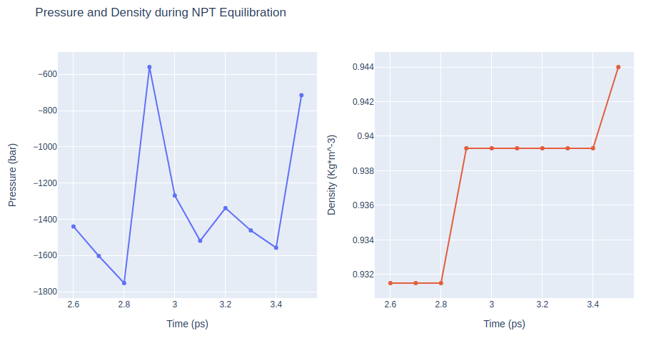
Equilibrate the system in NPT ensemble (constant number of particles -N-, Pressure -P-, and Temperature -T-), using the sander tool from the AMBER MD package. Upon completion of the previous equilibration steps, the system is now well-equilibrated at the desired temperature and pressure. The last step of the DNA MD setup is a short, free MD simulation, to ensure the robustness of the system.
AMBER MD configuration file used (step10.in) includes the following simulation parameters:
- imin = 0; Run MD (no minimization)
- nstlim = 500000; Number of MD steps
- dt = 0.002; Time step (in ps)
- ntx = 5; Read initial coordinates and velocities from restart file
- irest = 1; Restart previous simulation from restart file
- ig = -1; Seed for the pseudo-random number generator
- ntwx = 5000; Coordinates will be written to the output trajectory file every 5000 steps
- ntwv = -1; Velocities will be written to output trajectory file, making it a combined coordinate/velocity trajectory file, at the interval defined by ntwx
- ioutfm = 1; Write trajectory in netcdf format
- ntxo = 2; Write restart in netcdf format
- ntpr = 500; Write energy information to files 'mdout' and 'mdinfo' every 500 steps
- ntwr = 50000; Write information to restart file every 50000 steps
- iwrap = 0; Not wrapping coordinates into primary box
- nscm = 1000; Removing translational and rotational center-of-mass motions every 1000 steps
- ntc = 2; Turn on SHAKE for constraining length of bonds involving Hydrogen atoms
- ntf = 2; Force evaluation: Bond interactions involving H omitted (SHAKE)
- ntb = 2; Constant Pressure Periodic Boundary Conditions (PBC)
- cut = 9.0; Cutoff for non bonded interactions in Angstroms
- ntt = 3; Constant temperature using Langevin dynamics
- gamma_ln = 5; Collision frequency for Langevin dynamics (in 1/ps)
- temp0 = 310.0; Final temperature (310 K)
- tempi = 310.0; Initial temperature (310 K)
- ntp = 1; Constant pressure dynamics: md with isotropic position scaling
- barostat = 2; Monte Carlo Barostat
- pres0 = 1.0; Reference pressure at which the system is maintained
- ntr = 0; Turn off positional restraints
NPT equilibration step without any position restraints.
Removing translational and rotational center-of-mass motions. Timestep 2fs. Writing times changed (production MD).
Restarting from previous equilibration step.
Building Blocks used:
- sander_mdrun from biobb_amber.sander.sander_mdrun
- process_mdout from biobb_amber.process.process_mdout
# Import module
from biobb_amber.sander.sander_mdrun import sander_mdrun

# Create prop dict and inputs/outputs
prop = {
    "mdin" : {
        'nstlim' : 500,  # Overwrite number of MD steps if needed
        'ntpr' : 50      # Overwrite energy information writing frequency
    },
#    "sander_path" : "sander.MPI",  # Change sander binary to parallel (MPI) execution (not included in AmberTools)
#    "mpi_bin" : "mpirun",          # MPI runner
#    "mpi_np" : 16                  # Number of cores to use in the MPI parallel calculation
}
output_eq10_traj_path = 'sander.eq10.nc'
output_eq10_rst_path = 'sander.eq10.ncrst'
output_eq10_log_path = 'sander.eq10.log'
output_eq10_mdinfo_path = 'sander.eq10.mdinfo'

# Create and launch bb
sander_mdrun(input_top_path=dna_leap_top_4fs_path,
            input_mdin_path="ABCix_config_files/step10.in",
            input_crd_path=output_eq9_rst_path,
            input_ref_path=output_eq9_rst_path,
            output_traj_path=output_eq10_traj_path,
            output_rst_path=output_eq10_rst_path,
            output_log_path=output_eq10_log_path,
            output_mdinfo_path=output_eq10_mdinfo_path,
            properties=prop)
# Import module
from biobb_amber.process.process_mdout import process_mdout

# Create prop dict and inputs/outputs
prop = {
    "terms" : ['PRES','DENSITY']
}
output_dat_eq10_path = 'sander.eq10.pressure_and_density.dat'

# Create and launch bb
process_mdout(input_log_path=output_eq10_log_path,
            output_dat_path=output_dat_eq10_path,
            properties=prop)
# Read pressure and density data from file
import plotly.graph_objs as go
from plotly import subplots

# Read pressure and density data from file
with open(output_dat_eq10_path, 'r') as pd_file:
    x, y, z = zip(*[
        (float(line.split()[0]), float(line.split()[1]), float(line.split()[2]))
        for line in pd_file
        if not line.startswith(("#", "@"))
    ])

# Create a scatter plot
trace1 = go.Scatter(
    x=x,y=y
)
trace2 = go.Scatter(
    x=x,y=z
)

fig = subplots.make_subplots(rows=1, cols=2, print_grid=False)

fig.append_trace(trace1, 1, 1)
fig.append_trace(trace2, 1, 2)

fig['layout']['xaxis1'].update(title='Time (ps)')
fig['layout']['xaxis2'].update(title='Time (ps)')
fig['layout']['yaxis1'].update(title='Pressure (bar)')
fig['layout']['yaxis2'].update(title='Density (Kg*m^-3)')

fig['layout'].update(title='Pressure and Density during NPT Equilibration')
fig['layout'].update(showlegend=False)
fig['layout'].update(height=500)

# Show the figure (renderer changes for colab and jupyter)
rend = 'colab' if 'google.colab' in sys.modules else ''
fig.show(renderer=rend)
Free Molecular Dynamics Simulation
Upon completion of the 10 equilibration phases, the system can now be used for the production simulation.
In the ABCix run of the ABC consortium, a 4fs timestep is used, applying hydrogen-mass repartition. Langevin algorithm is used for the temperature coupling and Monte Carlo barostat algorithm for pressure coupling.
AMBER MD configuration file used (md.in) includes the following simulation parameters:
-
imin = 0; Run MD (no minimization)
-
nstlim = 500000; Number of MD steps -- 1ns
-
dt = 0.004; Time step (in ps) -- using H-mass repartition
-
ntx = 5; Read initial coordinates and velocities from restart file
-
irest = 1; Restart previous simulation from restart file
-
ig = -1; Seed for the pseudo-random number generator
-
ntpr = 5000; Write energy information to files 'mdout' and 'mdinfo' every 5000 steps -- 20ps
-
ntwr = 5000; Write information to restart file every 5000 steps -- 20ps
-
ntwx = 5000; Coordinates will be written to the output trajectory file every 5000 steps -- 20ps
-
ntc = 2; Turn on SHAKE for constraining length of bonds involving Hydrogen atoms
-
ntf = 2; Force evaluation: Bond interactions involving H omitted (SHAKE)
-
iwrap = 1; Wrapping coordinates into primary box
-
ntb = 2; Constant Pressure Periodic Boundary Conditions (PBC)
-
ntp = 1; Constant pressure dynamics: md with isotropic position scaling
-
barostat = 2; Monte Carlo Barostat
-
mcbarint = 100; Number of steps between volume change attempts performed as part of the Monte Carlo barostat
-
pres0 = 1.0; Reference pressure at which the system is maintained
-
cut = 8.0; Cutoff for non bonded interactions in Angstroms
-
temp0 = 310.0; Final temperature (310 K)
-
ntt = 3; Constant temperature using Langevin dynamics
-
gamma_ln = 0.01; Collision frequency for Langevin dynamics (in 1/ps)
-
tol = 0.0000001; Relative geometrical tolerance for coordinate resetting in shake
-
timlim = 170000; Time limit for the simulation
Note: Although not stated explicitly, all output files will be generated in binary netcdf format (default for ioutfm and ntxo parameters).
Building Blocks used:
- sander_mdrun from biobb_amber.sander.sander_mdrun
- process_mdout from biobb_amber.process.process_mdout
# Import module
from biobb_amber.sander.sander_mdrun import sander_mdrun

# Create prop dict and inputs/outputs
prop = {
    "mdin" : {
        'nstlim' : 500,  # Overwrite number of MD steps if needed
        'ntpr' : 50      # Overwrite energy information writing frequency
    },
#    "sander_path" : "sander.MPI",  # Change sander binary to parallel (MPI) execution (not included in AmberTools)
#    "mpi_bin" : "mpirun",          # MPI runner
#    "mpi_np" : 16                  # Number of cores to use in the MPI parallel calculation
}
output_md_traj_path = 'sander.md.nc'
output_md_rst_path = 'sander.md.ncrst'
output_md_log_path = 'sander.md.log'
output_md_mdinfo_path = 'sander.md.mdinfo'

# Create and launch bb
sander_mdrun(input_top_path=dna_leap_top_4fs_path,
            input_mdin_path="ABCix_config_files/md.in",
            input_crd_path=output_eq10_rst_path,
            input_ref_path=output_eq10_rst_path,
            output_traj_path=output_md_traj_path,
            output_rst_path=output_md_rst_path,
            output_log_path=output_md_log_path,
            output_mdinfo_path=output_md_mdinfo_path,
            properties=prop)
Output files
Important Output files generated:
- output_md_traj_path (sander.md.nc): Final trajectory of the MD setup protocol (netcdf).
- output_ions_top_path (structure.ions.parmtop): Final topology of the MD system.
- dna_leap_top_4fs_path (structure.leap.4fs.top): Final topology of the MD system with hydrogen mass repartition (allowing 4fs timestep).
- output_md_rst_path (sander.md.ncrst): Final restart file of the MD setup protocol (ncrst).
from IPython.display import FileLink
display(FileLink(output_md_traj_path))
display(FileLink(output_ions_top_path))
display(FileLink(dna_leap_top_4fs_path))
display(FileLink(output_md_rst_path))
