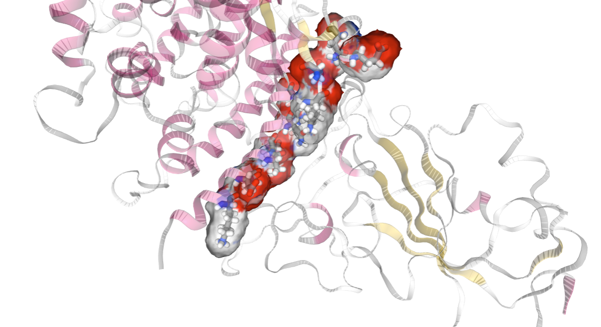
Molecular Interaction Potentials
Classical Molecular Interaction Potentials tutorial using BioExcel Building Blocks (biobb)
This tutorial aims to illustrate the process of computing classical molecular interaction potentials from protein structures, step by step, using the BioExcel Building Blocks library (biobb). Examples shown are Molecular Interaction Potentials (MIPs) grids, protein-protein/ligand interaction potentials, and protein titration. The particular structures used are the Lysozyme protein (PDB code 1AKI, https://doi.org/10.2210/pdb1AKI/pdb), the Epidermal Growth Factor Receptor kinase domain (PDB code 4HJO, https://doi.org/10.2210/pdb4HJO/pdb) complexed with the Erlotinib inhibitor (PDB code AQ4, DrugBank Ligand Code DB00530), and a MD simulation of the complex formed by the SARS-CoV-2 Receptor Binding Domain and the human Angiotensin Converting Enzyme 2 (PDB code 6VW1, https://doi.org/10.2210/pdb6VW1/pdb).
The code wrapped is the Classical Molecular Interaction Potentials (CMIP) code:
Classical molecular interaction potentials: Improved setup procedure in molecular dynamics simulations of proteins. Gelpí, J.L., Kalko, S.G., Barril, X., Cirera, J., de la Cruz, X., Luque, F.J. and Orozco, M. (2001) Proteins, 45: 428-437. https://doi.org/10.1002/prot.1159
Settings
Biobb modules used
- biobb_io: Tools to fetch biomolecular data from public databases.
- biobb_cmip: Tools to compute classical molecular interaction potentials from protein structures.
- biobb_structure_utils: Tools to modify or extract information from a PDB structure.
- biobb_chemistry: Tools to perform chemoinformatics on molecular structures.
- biobb_amber: Tools to setup and simulate atomistic MD simulations using AMBER MD package.
Auxiliary libraries used
- jupyter: Free software, open standards, and web services for interactive computing across all programming languages.
- nglview: Jupyter/IPython widget to interactively view molecular structures and trajectories in notebooks.
- plotly: Python interactive graphing library integrated in Jupyter notebooks.
- simpletraj: Lightweight coordinate-only trajectory reader based on code from GROMACS, MDAnalysis and VMD.
Conda Installation and Launch
git clone https://github.com/bioexcel/biobb_wf_cmip.git
cd biobb_wf_cmip
conda env create -f conda_env/environment.yml
conda activate biobb_wf_cmip
jupyter-notebook biobb_wf_cmip/notebooks/biobb_wf_cmip.ipynb
Pipeline steps
- Input Parameters
- Fetching PDB structure
- CMIP PDB preparation (from PDB structure)
- Structural water molecules & ions
- Molecular Interaction Potentials
- Interaction Potential Energies
- Questions & Comments

Initializing colab
The two cells below are used only in case this notebook is executed via Google Colab. Take into account that, for running conda on Google Colab, the condacolab library must be installed. As explained here, the installation requires a kernel restart, so when running this notebook in Google Colab, don't run all cells until this installation is properly finished and the kernel has restarted.
# Only executed when using google colab
import sys
if 'google.colab' in sys.modules:
  import subprocess
  from pathlib import Path
  try:
    subprocess.run(["conda", "-V"], check=True)
  except FileNotFoundError:
    subprocess.run([sys.executable, "-m", "pip", "install", "condacolab"], check=True)
    import condacolab
    condacolab.install()
    # Clone repository
    repo_URL = "https://github.com/bioexcel/biobb_wf_cmip.git"
    repo_name = Path(repo_URL).name.split('.')[0]
    if not Path(repo_name).exists():
      subprocess.run(["mamba", "install", "-y", "git"], check=True)
      subprocess.run(["git", "clone", repo_URL], check=True)
      print("⏬ Repository properly cloned.")
    # Install environment
    print("⏳ Creating environment...")
    env_file_path = f"{repo_name}/conda_env/environment.yml"
    subprocess.run(["mamba", "env", "update", "-n", "base", "-f", env_file_path], check=True)
    print("🎨 Install NGLView dependencies...")
    subprocess.run(["mamba", "install", "-y", "-c", "conda-forge", "nglview==3.0.8", "ipywidgets=7.7.2"], check=True)
    print("👍 Conda environment successfully created and updated.")
# Enable widgets for colab
if 'google.colab' in sys.modules:
  from google.colab import output
  output.enable_custom_widget_manager()
  # Change working dir
  import os
  os.chdir("biobb_wf_cmip/biobb_wf_cmip/notebooks")
  print(f"📂 New working directory: {os.getcwd()}")
Input parameters
Input parameters needed:
- pdbCode: PDB code of the protein structure (e.g. 1AKI, https://doi.org/10.2210/pdb1AKI/pdb)
- complexCode: PDB code of the protein-ligand complex (e.g. 4HJO [EGFR + Erlotinib], https://doi.org/10.2210/pdb4HJO/pdb)
- ligandCode: PDB code of the ligand (e.g. AQ4 [Erlotinib], DrugBank Ligand Code DB00530)
- mol_charge: Charge of the small molecule
-
MDCode: Code of the Molecular Dynamics trajectory (e.g. RBD-hACE2)
- inputPDB_MD: MD reference structure (PDB format)
- inputTOP_MD: MD topology (Amber Parmtop7 format)
import nglview
import ipywidgets
import plotly
import sys
from plotly import subplots
import plotly.graph_objs as go

pdbCode = "1aki"       # Structure of the orthorhombic form of Hen Egg-white Lysozyme
complexCode = "4hjo"   # Crystal structure of the inactive EGFR tyrosine kinase domain with erlotinib
ligandCode = "AQ4"     # Erlotinib epidermal growth factor receptor (EGFR) tyrosine kinase inhibitor
mol_charge = 0         # Molecular charge for Erlotinib

MDCode = "RBD-hACE2-ZN"
inputPDB_MD = "Files/" + MDCode + ".pdb" # Structure of the SARS-CoV-2 RBD-hACE2 complex
inputTOP_MD = "Files/" + MDCode + ".top" # MD Topology of the SARS-CoV-2 RBD-hACE2 complex
Fetching PDB structure
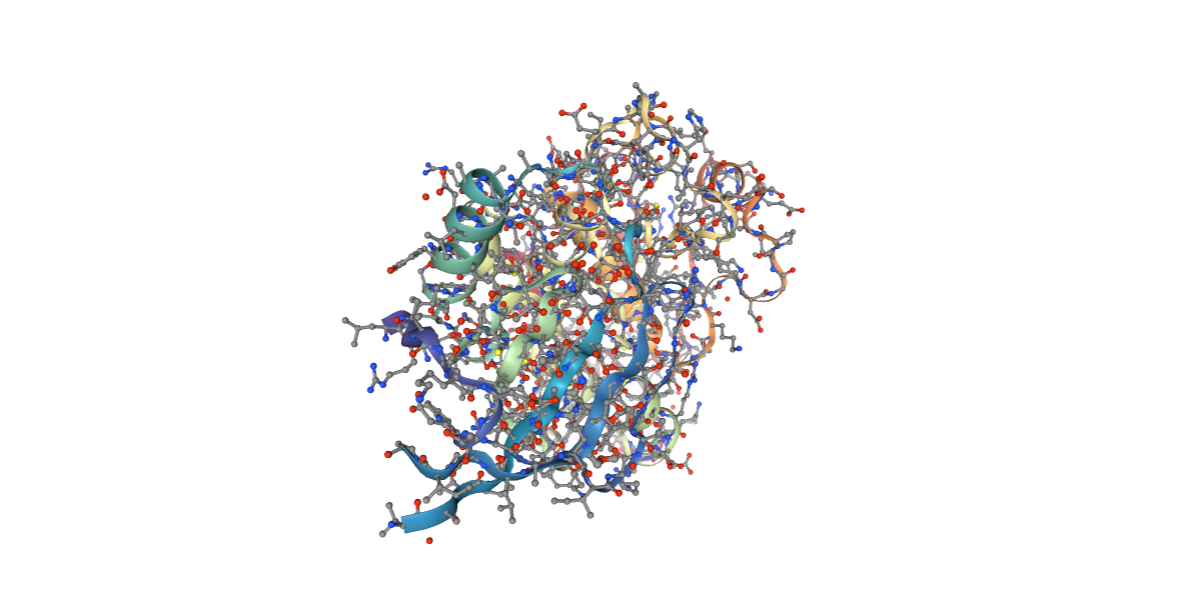
Downloading PDB structure with the protein molecule from the RCSB PDB database.
Alternatively, a PDB file can be used as starting structure.
Building Blocks used:
- Pdb from biobb_io.api.pdb
# Downloading desired PDB file
# Import module
from biobb_io.api.pdb import pdb

# Create properties dict and inputs/outputs
downloaded_pdb = pdbCode+'.pdb'
prop = {
    'pdb_code': pdbCode,
    'api_id' : 'mmb'
}

#Create and launch bb
pdb(output_pdb_path=downloaded_pdb,
    properties=prop)
# Show protein
view = nglview.show_structure_file(downloaded_pdb)
view.add_representation(repr_type='ball+stick', selection='all')
view._remote_call('setSize', target='Widget', args=['','600px'])
view
CMIP PDB Preparation (from PDB structure)
CMIP tool needs additional information (e.g. charges, elements) to be included in the structure PDB file to properly run. A specific BioBB building block (prepare_pdb) is used in the next cell to prepare the input PDB file, adding this extra information. Charges and elements are taken from an internal CMIP library based on the AMBER force fields.
Building Blocks used:
- cmip_prepare_pdb from biobb_cmip.cmip.cmip_prepare_pdb
from biobb_cmip.cmip.cmip_prepare_pdb import cmip_prepare_pdb

cmipPDB = pdbCode + ".cmip.pdb"

cmip_prepare_pdb(input_pdb_path=downloaded_pdb,
            output_cmip_pdb_path=cmipPDB
)
Structural water molecules & ions
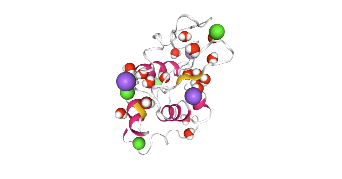
One of the many steps involved in the MD structure setup process is the addition of solvent and counterions (when working with explicit solvent). Solvent molecules and counterions are usually integrated on the structure surface in two steps:
- Structural waters/ions: A first shell of water molecules and ions is commonly added in the energetically most favorable positions on the surface of the structure. It is a computationally expensive process and is usually reduced to just tens of water molecules and ions (depending on the structure size).
- Solvent box/ionic concentration: A box of solvent molecules is created surrounding the original structure, and an additional number of ions are added until reaching a desired ionic concentration.
Whereas the second step is integrated in all the MD packages, the first one is rarely available. CMIP and the biobb_titration building block is helping in this task.
Building Blocks used:
- cmip_titration from biobb_cmip.cmip.cmip_titration
- cat_pdb from biobb_structure_utils.utils.cat_pdb
from biobb_cmip.cmip.cmip_titration import cmip_titration

wat_ions_pdb = pdbCode + ".wat_ions.pdb"
wat_ions_log = pdbCode + ".wat_ions.log"

prop = {
#    'neutral' : True, # Can be also used to neutralize the system
    'num_positive_ions' : 5,
    'num_negative_ions' : 5,
    'num_wats' : 20
}

cmip_titration(input_pdb_path=cmipPDB,
          input_vdw_params_path='/usr/local/share/cmip/dat/vdwprm' if 'google.colab' in sys.modules else None,
          output_pdb_path=wat_ions_pdb,
          output_log_path=wat_ions_log,
          properties=prop)
from biobb_structure_utils.utils.cat_pdb import cat_pdb

titPDB = pdbCode + ".tit.pdb"

cat_pdb(input_structure1=cmipPDB,
       input_structure2=wat_ions_pdb,
       output_structure_path=titPDB)
view = nglview.show_structure_file(titPDB)
view.clear_representations()
view.add_representation(repr_type='cartoon', selection='protein', color='sstruc')
view.add_representation(repr_type='spacefill', selection='water')
view.add_representation(repr_type='spacefill', selection='.Na', color='element')
view.add_representation(repr_type='spacefill', selection='.Cl', color='element')
view._remote_call('setSize', target='Widget', args=['','600px'])
view
Molecular Interaction Potentials (MIPs)
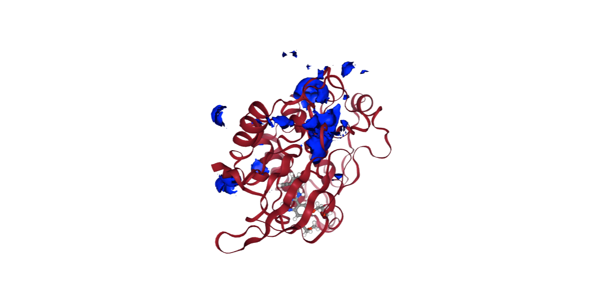
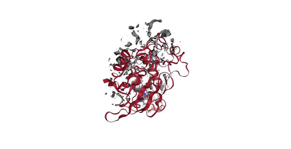
Molecular interaction potentials (MIP) are field properties arising from the interaction of a probe (e.g., methyl, proton or water) with a molecule. These are calculated in the surface of the molecule, with a grid defined around the structure.
MIPs are one of the most important molecular properties in the relationship between molecular and binding data (e.g. 3D Quantitative Structure-Activity Relationships, 3D-QSAR), and is extensively applied in drug discovery processes.
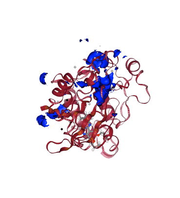
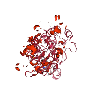
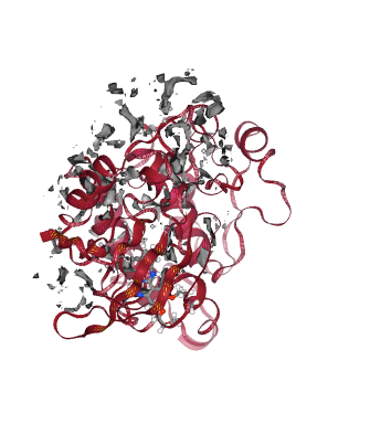
In this example, three different MIPs are used, with a Water Oxygen atom as a probe:
- Positive MIP - highlighting the protein regions with higher affinity to negatively charged groups.
- Negative MIP - highlighting the protein regions with higher affinity to positively charged groups.
- Neutral MIP - highlighting the protein regions with lower affinity to electrocharged groups.
Building Blocks used:
- cmip from biobb_cmip.cmip.cmip
from biobb_cmip.cmip.cmip_run import cmip_run

mip_pos_log = pdbCode + ".mip_pos.log"
mip_pos_cube = pdbCode + ".mip_pos.cube"

prop = {
    'execution_type' : 'mip_pos'
}

cmip_run( input_pdb_path=cmipPDB,
          input_vdw_params_path='/usr/local/share/cmip/dat/vdwprm' if 'google.colab' in sys.modules else None,
          output_log_path=mip_pos_log,
          output_cube_path=mip_pos_cube,
          properties=prop)
view = nglview.show_structure_file(mip_pos_cube)
view.add_component(nglview.FileStructure(cmipPDB))
view.clear_representations()
view.add_representation(repr_type='cartoon', selection='protein', color='sstruc')
view.add_surface(isolevelType="value", isolevel=-5, color="blue")
view.component_1.center()
view._remote_call('setSize', target='Widget', args=['','600px'])
view
from biobb_cmip.cmip.cmip_run import cmip_run

mip_neg_log = pdbCode + ".mip_neg.log"
mip_neg_cube = pdbCode + ".mip_neg.cube"

prop = {
    'execution_type' : 'mip_neg'
}

cmip_run(input_pdb_path=cmipPDB,
         input_vdw_params_path='/usr/local/share/cmip/dat/vdwprm' if 'google.colab' in sys.modules else None,
         output_log_path=mip_neg_log,
         output_cube_path=mip_neg_cube,
         properties=prop)
view = nglview.show_structure_file(mip_neg_cube)
view.add_component(nglview.FileStructure(cmipPDB))
view.clear_representations()
view.add_representation(repr_type='cartoon', selection='protein', color='sstruc')
view.add_surface(isolevelType="value", isolevel=-10, color="red")
view.component_1.center()
view._remote_call('setSize', target='Widget', args=['','600px'])
view

from biobb_cmip.cmip.cmip_run import cmip_run

mip_neutral_log = pdbCode + ".mip_neutral.log"
mip_neutral_cube = pdbCode + ".mip_neutral.cube"

prop = {
    'execution_type' : 'mip_neu'
}

cmip_run( input_pdb_path=cmipPDB,
          input_vdw_params_path='/usr/local/share/cmip/dat/vdwprm' if 'google.colab' in sys.modules else None,
          output_log_path=mip_neutral_log,
          output_cube_path=mip_neutral_cube,
          properties=prop)
view = nglview.show_structure_file(mip_neutral_cube)
view.add_component(nglview.FileStructure(cmipPDB))
view.clear_representations()
view.add_representation(repr_type='cartoon', selection='protein', color='sstruc')
view.add_surface(isolevelType="value", isolevel=-1, color="grey")
view.component_1.center()
view._remote_call('setSize', target='Widget', args=['','600px'])
view
#Show different structures generated (for comparison)
view1 = nglview.show_structure_file(cmipPDB)
view1.add_component(nglview.FileStructure(mip_pos_cube))
view1.component_0.add_representation(repr_type='cartoon', selection='protein', color='sstruc')
view1.component_1.add_surface(isolevelType="value", isolevel=-5, color="blue")
view1.component_0.center()
view1._remote_call('setSize', target='Widget', args=['350px','400px'])
view1.camera='orthographic'
view1
view2 = nglview.show_structure_file(cmipPDB)
view2.add_component(nglview.FileStructure(mip_neg_cube))
view2.component_0.add_representation(repr_type='cartoon', selection='protein', color='sstruc')
view2.component_1.add_surface(isolevelType="value", isolevel=-10, color="red")
view2.component_0.center()
view2._remote_call('setSize', target='Widget', args=['350px','400px'])
view2.camera='orthographic'
view2
view3 = nglview.show_structure_file(cmipPDB)
view3.add_component(nglview.FileStructure(mip_neutral_cube))
view3.component_0.add_representation(repr_type='cartoon', selection='protein', color='sstruc')
view3.component_1.add_surface(isolevelType="value", isolevel=-1, color="grey")
view3.component_0.center()
view3._remote_call('setSize', target='Widget', args=['350px','400px'])
view3.camera='orthographic'
view3
ipywidgets.HBox([view1, view2, view3])
Interaction Potential Energies
Closely related to the previous study of Molecular Interaction Potentials, the Interaction Potential Energies calculation computes the contributions to the total energy of the system from the different interactions between the subunits of the molecule considered. These interaction energies usually depend on the relation between the charge and positions of the units studied (e.g. electrostatic, van der Waals) and the solvation energy (energy released when a compound is dissolved in a solvent).
Interaction Potential Energies give useful insights in the macromolecular interaction process, with the possibility to identify key residues involved in the interaction, and thus being another key component of the drug discovery process.
To illustrate the calculation of the interaction potentials between two subunits of a structure complex (e.g. protein-protein, protein-ligand), two different examples are used:
- Epidermal Growth Factor Receptor kinase domain with Erlotinib inhibitor.
- SARS-CoV-2 Receptor Binding Domain with human Angiotensin Converting Enzyme 2.
Protein-Ligand Interaction Energies
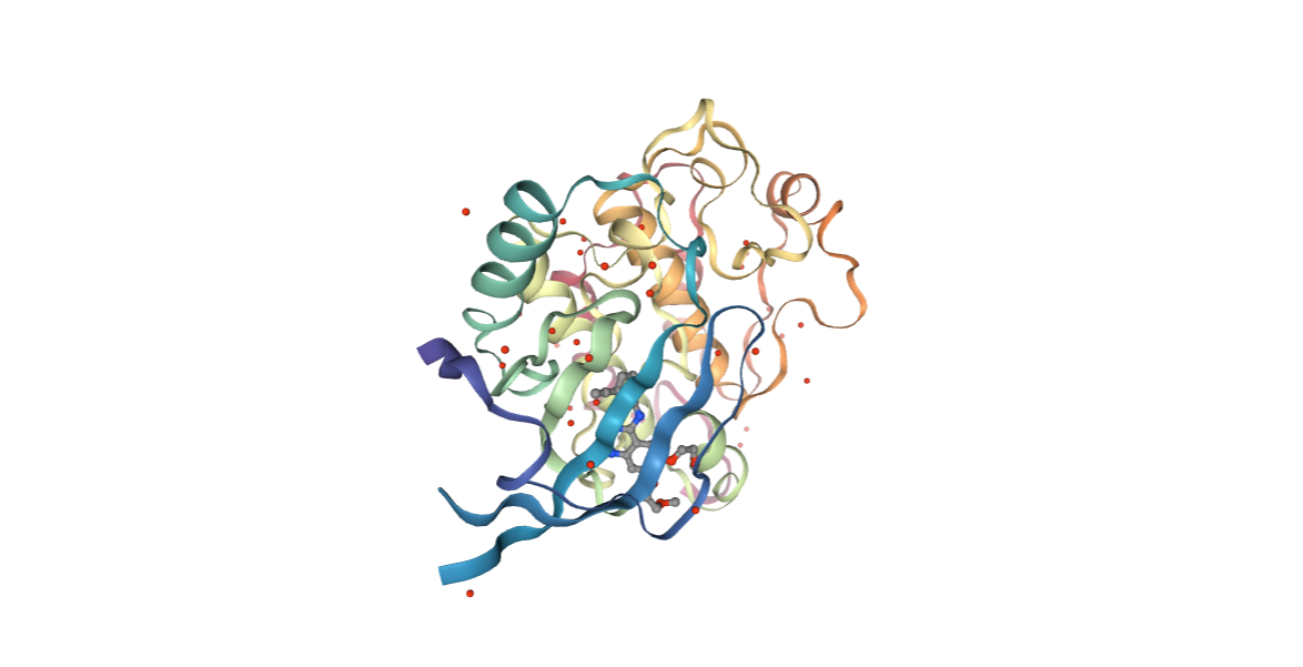
This example illustrates the steps needed to compute the protein-ligand interaction energies from a crystal structure of the complex taken directly from the PDB data bank. The particular example used is the Epidermal Growth Factor Receptor kinase domain (PDB code [4HJO](https://www.rcsb.org/structure/4HJO, https://doi.org/10.2210/pdb4HJO/pdb) with Erlotinib inhibitor (PDB code AQ4, DrugBank Ligand Code DB00530).
To properly compute the interaction energies, the protein-ligand complex needs to be pre-processed, adding the (typically) missing hydrogen atoms, finding out the atomic charges and elements, and relaxing the structure to avoid steric issues due to crystallographic packing. All these steps are performed in the following cells using BioBB building blocks
Fetching PDB structure
Downloading PDB structure with the protein molecule from the RCSB PDB database.
Alternatively, a PDB file can be used as starting structure.
Building Blocks used:
- Pdb from biobb_io.api.pdb
# Downloading desired PDB file
# Import module
from biobb_io.api.pdb import pdb

# Create properties dict and inputs/outputs
downloaded_pdb = complexCode+'.pdb'
prop = {
    'pdb_code': complexCode,
    'api_id' : 'mmb',
    'filter': ['ATOM', 'HETATM'],
}

#Create and launch bb
pdb(output_pdb_path=downloaded_pdb,
    properties=prop)
# Show protein
view = nglview.show_structure_file(downloaded_pdb)
view.add_representation(repr_type='ball+stick', selection='hetero')
view._remote_call('setSize', target='Widget', args=['','600px'])
view
Removing Water Molecules
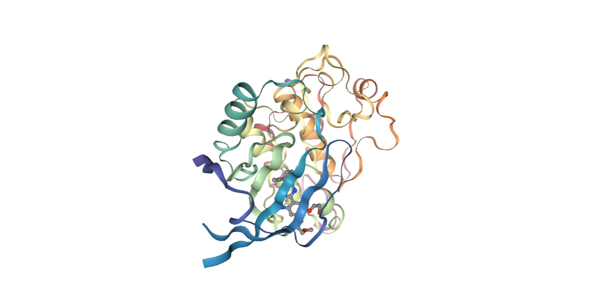
Removing the water molecules from the downloaded/given structure.
Building Blocks used:
- remove_pdb_water from biobb_structure_utils.utils
# Import module
from biobb_structure_utils.utils.remove_pdb_water import remove_pdb_water

# Removing Waters:

# Create properties dict and inputs/outputs
nohoh_pdb = complexCode+'.noHOH.pdb'

#Create and launch bb
remove_pdb_water(
    input_pdb_path=downloaded_pdb,
    output_pdb_path=nohoh_pdb
)
# Show protein
view = nglview.show_structure_file(nohoh_pdb)
view.add_representation(repr_type='ball+stick', selection='hetero')
view._remote_call('setSize', target='Widget', args=['','600px'])
view
Creating Ligand Topology
Obtaining parameters for the small molecule to be used in the potential energy calculations.
Building Blocks used:
- extract_heteroatoms from biobb_structure_utils.utils
- reduce_add_hydrogens from biobb_chemistry.ambertools
- acpype_params_ac from biobb_chemistry.acpype
# Create Ligand system topology, STEP 1
# Extracting Ligand
# Import module
from biobb_structure_utils.utils.extract_heteroatoms import extract_heteroatoms

# Create properties dict and inputs/outputs
ligandFile = ligandCode+'.pdb'

prop = {
     'heteroatoms' : [{"name": ligandCode}]
}

extract_heteroatoms(
    input_structure_path=nohoh_pdb,
    output_heteroatom_path=ligandFile,
    properties=prop
)
# Create Ligand system topology, STEP 2
# Reduce_add_hydrogens: add Hydrogen atoms to a small molecule (using Reduce tool from Ambertools package)
# Import module
from biobb_chemistry.ambertools.reduce_add_hydrogens import reduce_add_hydrogens

# Create prop dict and inputs/outputs
output_reduce_h = ligandCode+'.reduce.H.pdb'

# Create and launch bb
reduce_add_hydrogens(
    input_path=ligandFile,
    output_path=output_reduce_h
)
# Create Ligand system topology, STEP 3
# Acpype_params_gmx: Generation of topologies for AMBER with ACPype
# Import module
from biobb_chemistry.acpype.acpype_params_ac import acpype_params_ac

# Create prop dict and inputs/outputs
output_acpype_inpcrd = ligandCode+'params.inpcrd'
output_acpype_frcmod = ligandCode+'params.frcmod'
output_acpype_lib = ligandCode+'params.lib'
output_acpype_prmtop = ligandCode+'params.prmtop'
output_acpype = ligandCode+'params'

prop = {
    'basename' : output_acpype,
    'charge' : mol_charge
}

# Create and launch bb
acpype_params_ac(input_path=output_reduce_h,
                output_path_inpcrd=output_acpype_inpcrd,
                output_path_frcmod=output_acpype_frcmod,
                output_path_lib=output_acpype_lib,
                output_path_prmtop=output_acpype_prmtop,
                 properties=prop)
# Show different structures generated (for comparison)
view1 = nglview.show_structure_file(ligandFile)
view1.add_representation(repr_type='ball+stick')
view1._remote_call('setSize', target='Widget', args=['400px','400px'])
view1.camera='orthographic'
view1
view2 = nglview.show_structure_file(output_reduce_h)
view2.add_representation(repr_type='ball+stick')
view2._remote_call('setSize', target='Widget', args=['400px','400px'])
view2.camera='orthographic'
view2
ipywidgets.HBox([view1, view2])

Generating system topology
Generating the system topology for the protein-ligand complex using tleap from the AmberTools package. The topology will then be used to extract the needed parameters (e.g. atom charges) for the potential energy calculation.
Building Blocks used:
- leap_gen_top from biobb_amber.leap
# Import module
from biobb_amber.leap.leap_gen_top import leap_gen_top

# Create prop dict and inputs/outputs
output_pdb_path = 'structure.leap.pdb'
output_top_path = 'structure.leap.prmtop'
output_crd_path = 'structure.leap.crd'

prop = {
    "forcefield" : ["protein.ff14SB","gaff2"]
}

# Create and launch bb
leap_gen_top(input_pdb_path=nohoh_pdb,
           input_lib_path=output_acpype_lib,
           input_frcmod_path=output_acpype_frcmod,
           output_pdb_path=output_pdb_path,
           output_top_path=output_top_path,
           output_crd_path=output_crd_path,
           properties=prop)
Minimizing the energy of the system
Running a short energetic minimization to relax the system and remove possible clashes introduced by crystallographic constraints.
Building Blocks used:
- sander_mdrun from biobb_amber.sander
- amber_to_pdb from biobb_amber.ambpdb
from biobb_amber.sander.sander_mdrun import sander_mdrun

trj_amber = "structure.amber.crd"
rst_amber = "structure.amber.rst"
log_amber = "structure.amber.log"

prop = {
    'simulation_type' : 'minimization',
    'mdin' : {
        'ntb' : 0,        # Periodic Boundary. No periodicity is applied and PME (Particle Mesh Ewald) is off.
        'cut' : 12,       # Nonbonded cutoff, in Angstroms.
        'maxcyc' : 500,   # Maximum number of cycles of minimization.
        'ncyc' : 50,      # Minimization will be switched from steepest descent to conjugate gradient after ncyc cycles.
        'ntwx' : 50       # Trajectory output frequency
    }
}

sander_mdrun(
     input_top_path=output_top_path,
     input_crd_path=output_crd_path,
     output_traj_path=trj_amber,
     output_rst_path=rst_amber,
     output_log_path=log_amber,
     properties=prop
)
from biobb_amber.ambpdb.amber_to_pdb import amber_to_pdb

pdb_amber_min = "structure.amber-min.pdb"

amber_to_pdb(
      input_top_path=output_top_path,
      input_crd_path=rst_amber,
      output_pdb_path=pdb_amber_min
)
Preparing the structures for CMIP
Preparing the structures for the CMIP calculations, using the energetically relaxed PDB structure coordinates and the information from the generated topology. Files needed are:
- Protein-ligand Complex: Protein-Ligand complex, with information needed by CMIP (charges, elements)
- Protein isolated: Structure of the protein in apo state (without the ligand)
- Protein-ligand Complex with protein structure in dielectric mode (charges neutralized); Atoms in dielectric mode are occupying a volume but charges are replaced by a continuum dielectric, important for the interaction energy calculation. These atoms are identified by CMIP with an "X" letter just before the element symbol in the input PDB file (automatically inserted by the ignore_residues building block)
Building Blocks used:
- cmip_prepare_structure from biobb_cmip.cmip.cmip_prepare_structure
- remove_ligand from biobb_structure_utils.utils.remove_ligand
- cmip_ignore_residues from biobb_cmip.cmip.cmip_ignore_residues
from biobb_cmip.cmip.cmip_prepare_structure import cmip_prepare_structure

cmipPDB = complexCode + ".cmip.pdb"

cmip_prepare_structure(input_pdb_path=pdb_amber_min,
            input_topology_path=output_top_path,
            output_cmip_pdb_path=cmipPDB
)
# Import module
from biobb_structure_utils.utils.remove_ligand import remove_ligand

# Create properties dict and inputs/outputs
cmipPDB_EGFR_Prot = complexCode+'.noLIG.pdb'

prop = {
    'ligand' : ligandCode
}

#Create and launch bb
remove_ligand(input_structure_path=cmipPDB,
    output_structure_path=cmipPDB_EGFR_Prot,
    properties=prop)
CMIP PDB structure Preparation 3
Creating the Protein-ligand Complex with protein structure in dielectric mode. For this, all residues belonging to the protein structure (in this case, residues with id from 1 to 279) are marked with an 'X' symbol in the PDB. This is done by the ignore_residues building block.
from biobb_cmip.cmip.cmip_ignore_residues import cmip_ignore_residues

cmipPDB_EGFR_Prot_ignored = complexCode + ".Prot_ignored.cmip.pdb"

protein_residues = list(range(1,279))

prop = {
    'residue_list': protein_residues # WARNING: Change residue number accordingly
}

cmip_ignore_residues(input_cmip_pdb_path = cmipPDB,
                     output_cmip_pdb_path = cmipPDB_EGFR_Prot_ignored,
                     properties = prop)
Computing the Protein-Ligand interaction energies
Computing the Protein-Ligand interaction energies using the complex with the protein in dielectric mode as a CMIP host structure and the protein structure as a CMIP ligand (probe).
Building Blocks used:
- cmip from biobb_cmip.cmip.cmip
from biobb_cmip.cmip.cmip_run import cmip_run

EGFR_energies_log = complexCode + ".EGFR.energies.log"
EGFR_byat_out = complexCode + ".EGFR.energies.byat.out"

prop = {
    'execution_type' : 'pb_interaction_energy'
}

cmip_run(input_pdb_path=cmipPDB_EGFR_Prot_ignored,
         input_probe_pdb_path=cmipPDB_EGFR_Prot,
         input_vdw_params_path='/usr/local/share/cmip/dat/vdwprm' if 'google.colab' in sys.modules else None,
         output_log_path=EGFR_energies_log,
         output_byat_path=EGFR_byat_out,
         properties=prop)
Plotting the Protein-Ligand interaction energies by atom
Plotting the Protein-Ligand interaction energies with the protein atom id in the x-axis and the potential energies in KCal/mol in the y-axis. An auxiliary function included in the biobb_cmip module is used to extract the energies by atom (get_energies_byat).
import plotly.graph_objs as go
from biobb_cmip.utils.representation import get_energies_byat

atom_list, energy_dict = get_energies_byat(EGFR_byat_out, cutoff=50)

# Create a scatter plot
fig = go.Figure(data=go.Scatter(x=atom_list, y=energy_dict['ES&VDW'], mode='lines'))

# Update layout
fig.update_layout(title="CMIP Interaction Potential",
                  xaxis_title="Atom Number",
                  yaxis_title="Potential Energy Kcal/mol",
                  height=600)

# Show the figure (renderer changes for colab and jupyter)
rend = 'colab' if 'google.colab' in sys.modules else ''
fig.show(renderer=rend)

Plotting the Protein-Ligand interaction energies by residue
Plotting the Protein-Ligand interaction energies with the protein residue sequence in the x-axis and the potential energies in KCal/mol in the y-axis. An auxiliary function included in the biobb_cmip module is used to extract the energies by residues (get_energies_byres).
import plotly.graph_objs as go
import re
from biobb_cmip.utils.representation import get_energies_byres

res_list, energy_dict = get_energies_byres(EGFR_byat_out, cutoff=55)

# Create a scatter plot
fig = go.Figure(data=go.Scatter(x=res_list, y=energy_dict['ES&VDW'], mode='lines'))

# Update layout
fig.update_layout(title="CMIP Interaction Potential",
                  xaxis_title="Residue ID",
                  yaxis_title="Potential Energy Kcal/mol",
                  height=600)

# Show the figure (renderer changes for colab and jupyter)
rend = 'colab' if 'google.colab' in sys.modules else ''
fig.show(renderer=rend)

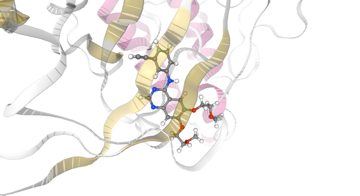
energy_cutoff = -1.5
identified_residues = [res_list[energy_dict['ES&VDW'].index(item)]
                       for item in energy_dict['ES&VDW'] if item < energy_cutoff]
identified_residues_ngl = str([int(re.sub(r'[A-Z]+ ', '', item)) for item in identified_residues]).replace(',','')

print ("Residues involved in the interaction (energy < " + str(energy_cutoff) + " KCal/mol):")
print (identified_residues_ngl)

# Show protein
view = nglview.show_structure_file(cmipPDB)
view.clear_representations()
view.add_representation(repr_type='cartoon', selection='all',color='sstruc',opacity=0.3)
view.add_representation(repr_type='ball+stick', selection=ligandCode)
view.add_representation(repr_type='licorice', selection=identified_residues_ngl)
view.center(ligandCode)
view._remote_call('setSize', target='Widget', args=['','600px'])
view
Protein-Protein Interaction Energies
This example illustrates the steps needed to compute the protein-protein interaction energies from a structure conformation of the complex taken directly from a Molecular Dynamics simulation. The particular example used is the SARS-CoV-2 Receptor Binding Domain (RBD) complexed with the human Angiotensin Converting Enzyme 2 (hACE2) (PDB code 6VW1, MD code MCV1900410, https://doi.org/10.2210/pdb6VW1/pdb).
view = nglview.show_structure_file(inputPDB_MD)
view.clear_representations()
view.add_representation(repr_type='cartoon', selection='protein', color='chainname')
view._remote_call('setSize', target='Widget', args=['','400px'])
view

CMIP PDB Preparation (from Molecular Dynamics topology)
When working with structure conformations taken from MD simulations, it is recommended to use the charges, atom types and elements considered in the simulation. Usually this information is stored in the so-called topology files. A specific building block (prepare_structure) is available to extract these information from an MD topology file and use it for the CMIP calculations.
The next cells are taking one frame of the MD simulation, splitting the subunits (chains) in two different PDB files, and preparing them to be used in CMIP, taking the charges and elements used in the simulations from the MD topology file.
Building Blocks used:
- prepare_structure from biobb_cmip.cmip.prepare_structure
- extract_chain from biobb_structure_utils.utils.extract_chain
from biobb_cmip.cmip.cmip_prepare_structure import cmip_prepare_structure

cmipPDB_MD = MDCode + ".cmip.pdb"

cmip_prepare_structure(input_pdb_path=inputPDB_MD,
                       input_topology_path=inputTOP_MD,
                       output_cmip_pdb_path=cmipPDB_MD)
from biobb_structure_utils.utils.extract_chain import extract_chain

cmipPDB_MD_hACE2 = MDCode + ".hACE2.cmip.pdb"
cmipPDB_MD_RBD = MDCode + ".RBD.cmip.pdb"

prop = {
    'chains': [ 'A' ],
    'permissive' : True
}
extract_chain(input_structure_path=cmipPDB_MD,
            output_structure_path=cmipPDB_MD_hACE2,
            properties=prop)

prop = {
    'chains': [ 'B' ],
    'permissive' : True
}
extract_chain(input_structure_path=cmipPDB_MD,
            output_structure_path=cmipPDB_MD_RBD,
            properties=prop)
# Show different structures generated
view1 = nglview.show_structure_file(cmipPDB_MD_hACE2)
view1.component_0.add_representation(repr_type='cartoon', selection='protein', color='sstruc')
view1.component_0.center()
view1._remote_call('setSize', target='Widget', args=['400px','400px'])
view1.camera='orthographic'
view1
view2 = nglview.show_structure_file(cmipPDB_MD_RBD)
view2.component_0.add_representation(repr_type='cartoon', selection='protein', color='sstruc')
view2.component_0.center()
view2._remote_call('setSize', target='Widget', args=['400px','400px'])
view2.camera='orthographic'
view2
ipywidgets.HBox([view1, view2])

CMIP Boxes
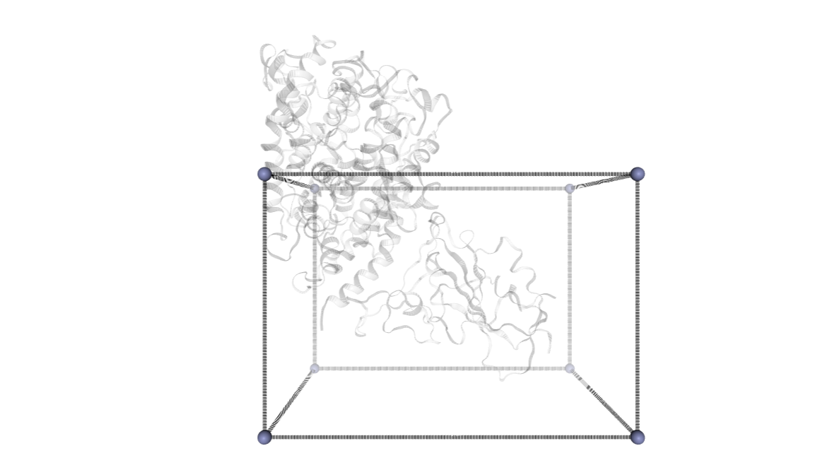
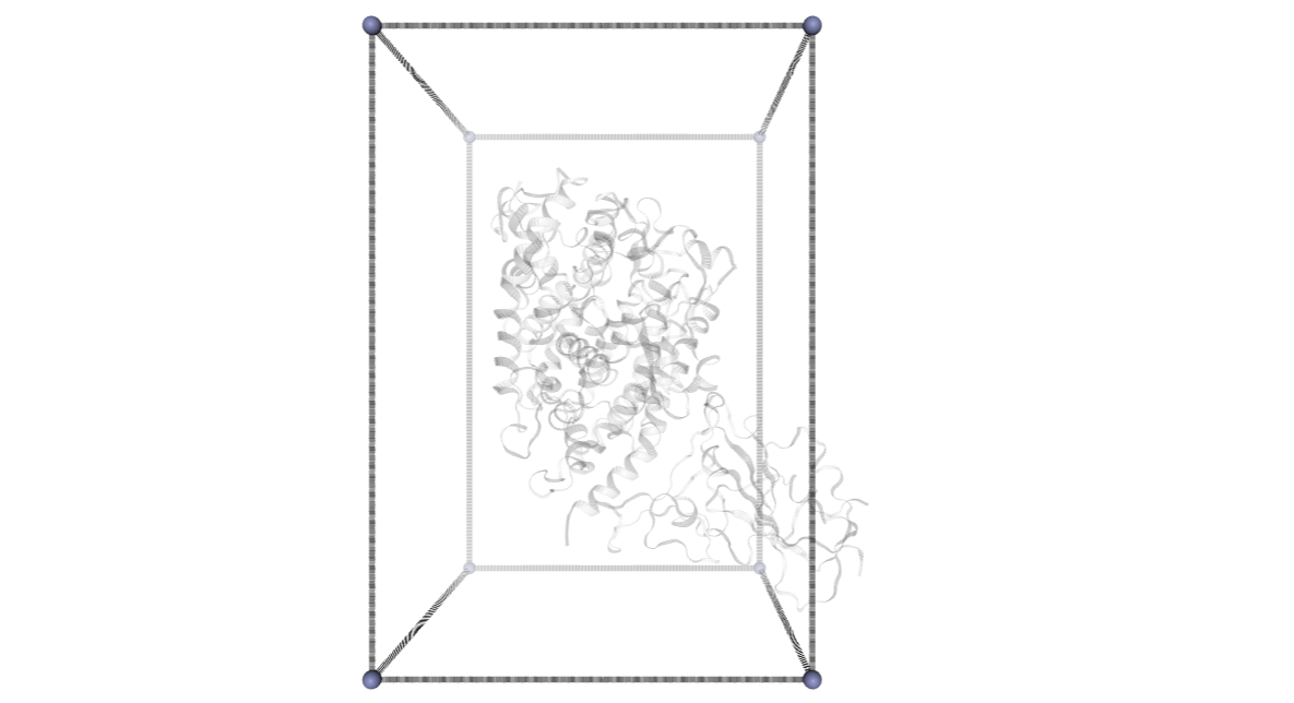
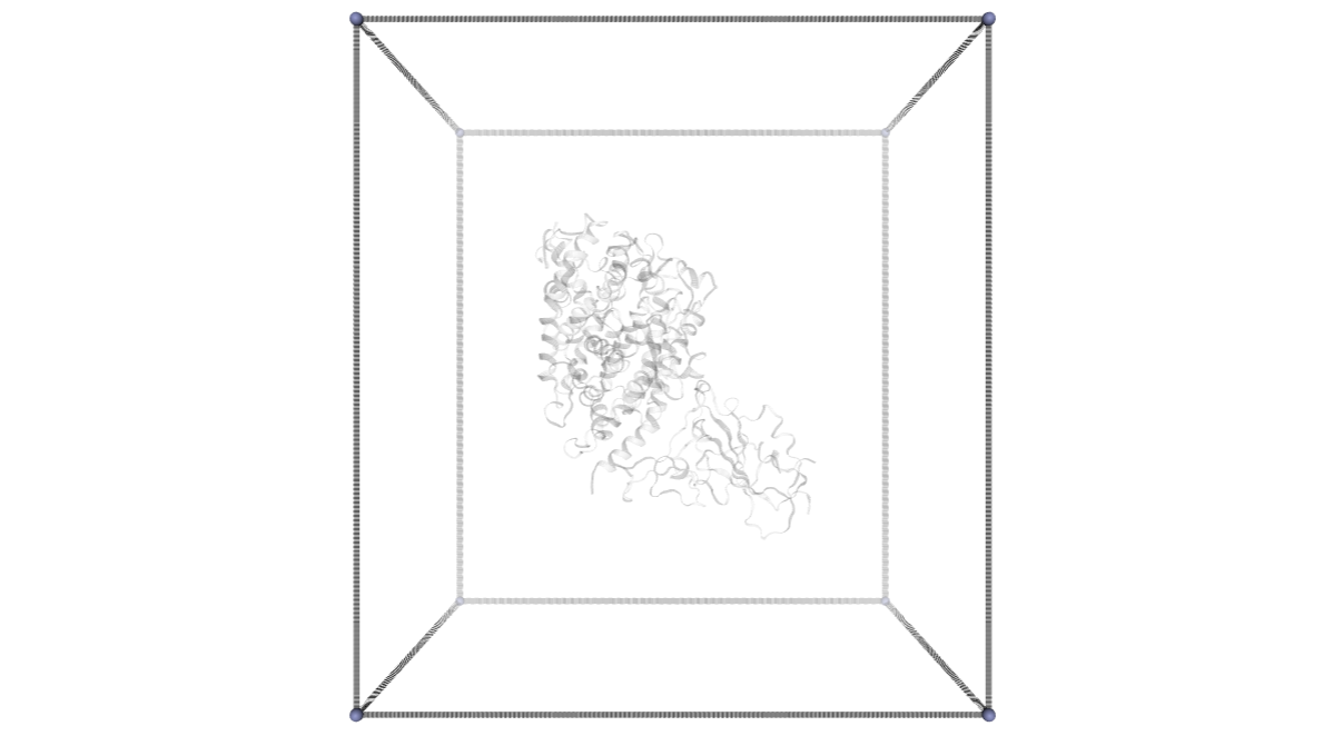
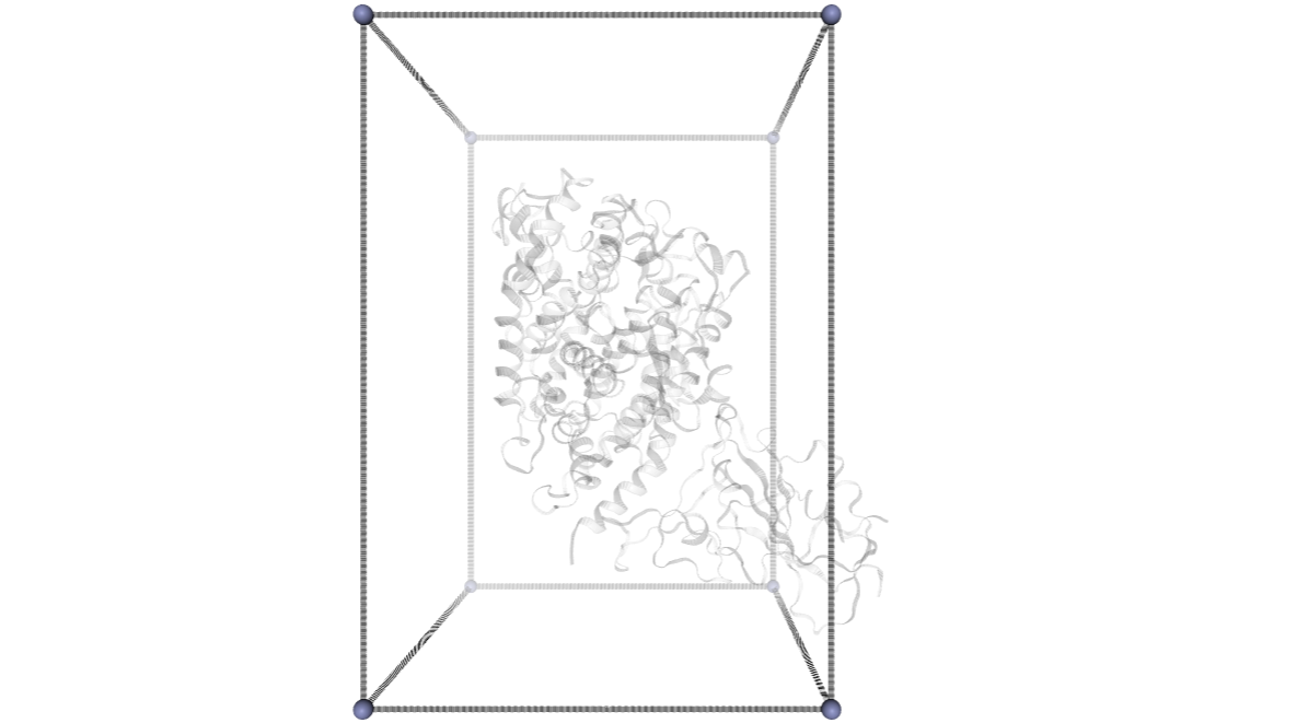
CMIP computes interaction energies using 3D grids (see image). CMIP tries to automatically built a grid enclosing the structure under study, which is fine in most of the cases. However, when working with protein-protein interactions, the grid needs to be adjusted to the system. The next cells are computing and showing the 3D grids needed to enclose the two monomers and the complex, and are useful to inspect them and re-define them, increasing the size, if needed.
A specific property of the cmip building block (execution_type = check_only) allows the calculation of the 3D grids, and accepts params such as perfill, which specifies the portion of the grid filled by the input (host) structure or box_size_factor, which increases the size of the grid. The computed grids can be then used as an input for the final interaction energies calculations.

Building Blocks used:
- cmip_run from biobb_cmip.cmip.cmip_run
from biobb_cmip.cmip.cmip_run import cmip_run

cmip_RBD_box_log = "RBD.box.log"
cmip_RBD_box_out = "RBD.box.byat.out"
cmip_RBD_box_json = "RBD.box.json"

prop = {
    'execution_type' : 'check_only',
    'params' : {
         'perfill' : 0.8
    }
}

cmip_run(input_pdb_path=cmipPDB_MD_RBD,
         input_vdw_params_path='/usr/local/share/cmip/dat/vdwprm' if 'google.colab' in sys.modules else None,
         output_log_path=cmip_RBD_box_log,
         output_json_box_path=cmip_RBD_box_json,
         properties=prop)
import nglview as nv
from biobb_cmip.utils.representation import create_box_representation

boxedFilename, atomPair = create_box_representation(cmip_RBD_box_log, inputPDB_MD)
# Represent the new file in ngl
view = nv.show_structure_file(boxedFilename, default=False)
# Structure
view.add_representation(repr_type='cartoon', selection='not het', color='#cccccc', opacity=.2)
# vertices box
view.add_representation(repr_type='ball+stick', selection='9999', aspectRatio = 10)
# lines box
view.add_representation(repr_type='distance', atomPair= atomPair, labelColor= 'transparent', color= 'black')
view.center()
view._remote_call('setSize', target='Widget', args=['','600px'])
view
from biobb_cmip.cmip.cmip_run import cmip_run

cmip_hACE2_box_log = "hACE2.box.log"
cmip_hACE2_box_out = "hACE2.box.byat.out"
cmip_hACE2_box_json = "hACE2.box.json"

prop = {
    'execution_type' : 'check_only',
    'params' : {
         'perfill' : 0.8,
    }
}

cmip_run(input_pdb_path=cmipPDB_MD_hACE2,
         input_vdw_params_path='/usr/local/share/cmip/dat/vdwprm' if 'google.colab' in sys.modules else None,
         output_log_path=cmip_hACE2_box_log,
         output_json_box_path=cmip_hACE2_box_json,
         properties=prop)
import nglview as nv
from biobb_cmip.utils.representation import create_box_representation

boxedFilename, atomPair = create_box_representation(cmip_hACE2_box_log, inputPDB_MD)
# Represent the new file in ngl
view = nv.show_structure_file(boxedFilename, default=False)
# Structure
view.add_representation(repr_type='cartoon', selection='not het', color='#cccccc', opacity=.2)
# vertices box
view.add_representation(repr_type='ball+stick', selection='9999', aspectRatio = 10)
# lines box
view.add_representation(repr_type='distance', atomPair= atomPair, labelColor= 'transparent', color= 'black')
view.center()
view._remote_call('setSize', target='Widget', args=['','600px'])
view
from biobb_cmip.cmip.cmip_run import cmip_run

cmip_COMPLEX_box_log = "COMPLEX.box.log"
cmip_COMPLEX_box_out = "COMPLEX.box.byat.out"
cmip_COMPLEX_box_json = "COMPLEX.box.json"

prop = {
    'execution_type' : 'check_only',
    'params' : {
         'perfill' : 0.6,
    }
}

cmip_run(input_pdb_path=cmipPDB_MD,
         input_vdw_params_path='/usr/local/share/cmip/dat/vdwprm' if 'google.colab' in sys.modules else None,
         output_log_path=cmip_COMPLEX_box_log,
         output_json_box_path=cmip_COMPLEX_box_json,
         properties=prop)
import nglview as nv
from biobb_cmip.utils.representation import create_box_representation

boxedFilename, atomPair = create_box_representation(cmip_COMPLEX_box_log, inputPDB_MD)
# Represent the new file in ngl
view = nv.show_structure_file(boxedFilename, default=False)
# Structure
view.add_representation(repr_type='cartoon', selection='not het', color='#cccccc', opacity=.2)
# vertices box
view.add_representation(repr_type='ball+stick', selection='9999', aspectRatio = 10)
# lines box
view.add_representation(repr_type='distance', atomPair= atomPair, labelColor= 'transparent', color= 'black')
view.center()
view._remote_call('setSize', target='Widget', args=['','600px'])
view

RDB Interaction Potential Energies
The first analysis computes the interaction potential energies for the RBD atoms with respect to the hACE2 enzyme.
Building Blocks used:
- cmip_ignore_residues from biobb_cmip.cmip.cmip_ignore_residues
- cmip_run from biobb_cmip.cmip.cmip_run
from biobb_cmip.cmip.cmip_ignore_residues import cmip_ignore_residues

cmipPDB_MD_RBD_ignored = MDCode + ".RBD_ignored.cmip.pdb"

prop = {
    'residue_list': "B:"
}

cmip_ignore_residues(input_cmip_pdb_path = cmipPDB_MD,
               output_cmip_pdb_path = cmipPDB_MD_RBD_ignored,
               properties = prop)
Computing the Protein-Protein interaction energies
Computing the Protein-Protein interaction energies using the RBD-hACE2 complex with the RBD in dielectric mode as a CMIP host structure and the RBD as a CMIP ligand (probe).
Grids sizes previously computed for the RBD (input_json_box_path) and for the RBD-hACE2 complex (input_json_external_box_path) are used as input information for the CMIP calculation.
from biobb_cmip.cmip.cmip_run import cmip_run

RBD_energies_log = "RBD.energies.log"
RBD_byat_out = "RBD.energies.byat.out"
output_RBD_box_json = "RBD.energies.box.output.json"
output_COMPLEX_box_json = "COMPLEX.energies.box.output.json"

prop = {
    'execution_type' : 'pb_interaction_energy'
}

cmip_run(input_pdb_path=cmipPDB_MD_RBD_ignored,
         input_probe_pdb_path=cmipPDB_MD_RBD,
         input_json_box_path=cmip_RBD_box_json,
         input_json_external_box_path=cmip_COMPLEX_box_json,
         input_vdw_params_path='/usr/local/share/cmip/dat/vdwprm' if 'google.colab' in sys.modules else None,
         output_json_box_path=output_RBD_box_json,
         output_json_external_box_path=output_COMPLEX_box_json,
         output_log_path=RBD_energies_log,
         output_byat_path=RBD_byat_out,
         properties=prop)
import nglview as nv
from biobb_cmip.utils.representation import create_box_representation

boxedFilename, atomPair = create_box_representation(output_COMPLEX_box_json, inputPDB_MD)
# Represent the new file in ngl
view = nv.show_structure_file(boxedFilename, default=False)
# Structure
view.add_representation(repr_type='cartoon', selection='not het', color='#cccccc', opacity=.2)
# vertices box
view.add_representation(repr_type='ball+stick', selection='9999', aspectRatio = 10)
# lines box
view.add_representation(repr_type='distance', atomPair= atomPair, labelColor= 'transparent', color= 'black')
view.center()
view._remote_call('setSize', target='Widget', args=['','600px'])
view
import plotly.graph_objs as go
from biobb_cmip.utils.representation import get_energies_byat

atom_list, energy_dict = get_energies_byat(RBD_byat_out, cutoff=55)

# Create a scatter plot
fig = go.Figure(data=go.Scatter(x=atom_list, y=energy_dict['ES&VDW'], mode='lines'))

# Update layout
fig.update_layout(title="CMIP Interaction Potential",
                  xaxis_title="Atom Number",
                  yaxis_title="Potential Energy Kcal/mol",
                  height=600)

# Show the figure (renderer changes for colab and jupyter)
rend = 'colab' if 'google.colab' in sys.modules else ''
fig.show(renderer=rend)

Interaction energies by residue
Visualizing the interaction potential energies computed by CMIP. The plot shows interactions energies (in kcal/mol, Y axis) for each of the residues (computed summing the contributions of all atoms included in the residue) of the RBD protein (X axis).
NOTE: This plot reproduces the analysis (for one single snapshot) presented here: https://bioexcel-cv19.bsc.es/#/id/MCV1900002/energies with Host: RBD and Guest: hACE2
import plotly.graph_objs as go
from biobb_cmip.utils.representation import get_energies_byres

res_list, energy_dict = get_energies_byres(RBD_byat_out, cutoff=55)

# Create a scatter plot
fig = go.Figure(data=go.Scatter(x=res_list, y=energy_dict['ES&VDW'], mode='lines'))

# Update layout
fig.update_layout(title="CMIP Interaction Potential",
                  xaxis_title="Residue ID",
                  yaxis_title="Potential Energy Kcal/mol",
                  height=600)

# Show the figure (renderer changes for colab and jupyter)
rend = 'colab' if 'google.colab' in sys.modules else ''
fig.show(renderer=rend)

energy_cutoff = -2
identified_residues = [res_list[energy_dict['ES&VDW'].index(item)]
                       for item in energy_dict['ES&VDW'] if item < energy_cutoff]
identified_residues_ngl = str([int(re.sub(r'[A-Z]+', '', item)) for item in identified_residues]).replace(',','')

print ("Residues involved in the interaction (energy < " + str(energy_cutoff) + " KCal/mol):")
print (identified_residues_ngl)

Visualizing the RBD residues involved in the interaction with hACE2
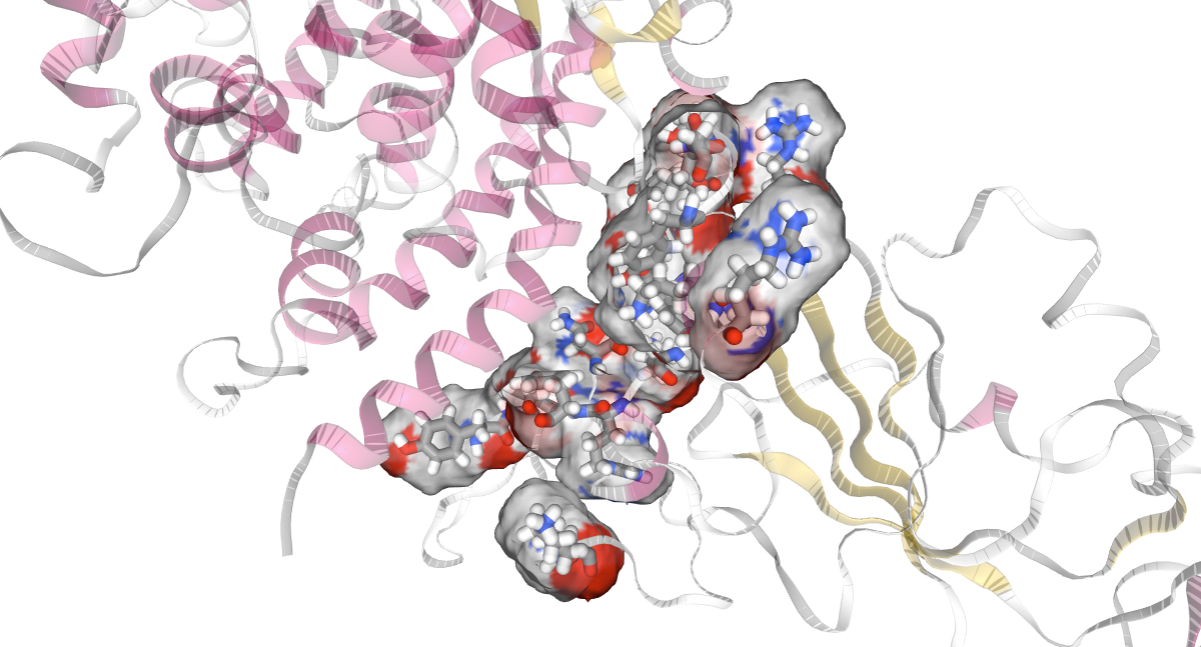
Viewing the RBD residues involved in the interaction with NGL. Residues in the interaction are represented in CPK (Ball & Sticks). Residues involved in the interaction have been selected in the previous cell as the ones having an interaction energy lower than a particular cutoff (-2 Kcal/mol). The cutoff can be changed to adapt it to the particular system.
# Show protein
view = nglview.show_structure_file(cmipPDB_MD)
view.clear_representations()
view.add_representation(repr_type='cartoon', selection='all',color='sstruc',opacity=0.3)
view.add_representation(repr_type='licorice', radius='0.5', selection=identified_residues_ngl)
view.add_representation(repr_type='surface', selection=identified_residues_ngl, opacity=0.2, color='element')
view.center(identified_residues_ngl)
view._remote_call('setSize', target='Widget', args=['','600px'])
view
hACE2 Interaction Potential Energies
The second analysis computes the interaction potential energies for the hACE2 atoms with respect to the RBD receptor.
Building Blocks used:
- cmip_ignore_residues from biobb_cmip.cmip.cmip_ignore_residues
- cmip_run from biobb_cmip.cmip.cmip_run
from biobb_cmip.cmip.cmip_ignore_residues import cmip_ignore_residues

cmipPDB_MD_hACE2_ignored = MDCode + ".hACE2_ign.cmip.pdb"

prop = {
    'residue_list': "A:"
}

cmip_ignore_residues(input_cmip_pdb_path = cmipPDB_MD,
                     output_cmip_pdb_path = cmipPDB_MD_hACE2_ignored,
                     properties = prop)
Computing the Protein-Protein interaction energies
Computing the Protein-Protein interaction energies using the complex with the hACE2 in dielectric mode as a CMIP host structure and the hACE2 as a CMIP ligand (probe).
Grids sizes previously computed for the hACE2 (input_json_box_path) and for the RBD-hACE2 complex (input_json_external_box_path) are used as input information for the CMIP calculation.
from biobb_cmip.cmip.cmip_run import cmip_run

hACE2_energies_log = "hACE2.energies.log"
hACE2_byat_out = "hACE2.energies.byat.out"
output_hACE2_box_json = "hACE2.energies.box.output.json"
output_COMPLEX_2_box_json = "COMPLEX_2.energies.box.output.json"

prop = {
    'execution_type' : 'pb_interaction_energy'
}

cmip_run(input_pdb_path=cmipPDB_MD_hACE2_ignored,
         input_probe_pdb_path=cmipPDB_MD_hACE2,
         input_json_box_path=cmip_hACE2_box_json,
         input_json_box_external_path=cmip_COMPLEX_box_json,
         input_vdw_params_path='/usr/local/share/cmip/dat/vdwprm' if 'google.colab' in sys.modules else None,
         output_json_box_path=output_hACE2_box_json,
         output_json_external_box_path=output_COMPLEX_2_box_json,
         output_log_path=hACE2_energies_log,
         output_byat_path=hACE2_byat_out,
         properties=prop)
import nglview as nv
from biobb_cmip.utils.representation import create_box_representation

boxedFilename, atomPair = create_box_representation(hACE2_energies_log, inputPDB_MD)
# Represent the new file in ngl
view = nv.show_structure_file(boxedFilename, default=False)
# Structure
view.add_representation(repr_type='cartoon', selection='not het', color='#cccccc', opacity=.2)
# vertices box
view.add_representation(repr_type='ball+stick', selection='9999', aspectRatio = 10)
# lines box
view.add_representation(repr_type='distance', atomPair= atomPair, labelColor= 'transparent', color= 'black')
view.center()
view._remote_call('setSize', target='Widget', args=['','600px'])
view
import plotly.graph_objs as go
from biobb_cmip.utils.representation import get_energies_byat

atom_list, energy_dict = get_energies_byat(hACE2_byat_out, cutoff=55)

# Create a scatter plot
fig = go.Figure(data=go.Scatter(x=atom_list, y=energy_dict['ES&VDW'], mode='lines'))

# Update layout
fig.update_layout(title="CMIP Interaction Potential",
                  xaxis_title="Atom Number",
                  yaxis_title="Potential Energy Kcal/mol",
                  height=600)

# Show the figure (renderer changes for colab and jupyter)
rend = 'colab' if 'google.colab' in sys.modules else ''
fig.show(renderer=rend)

Interaction energies by residue
Visualizing the interaction potential energies computed by CMIP. The plot shows interactions energies (in kcal/mol, Y axis) for each of the residues (computed summing the contributions of all atoms included in the residue) of the hACE2 protein (X axis).
NOTE: This plot reproduces the analysis (for one single snapshot) presented here: https://bioexcel-cv19.bsc.es/#/id/MCV1900002/energies with Host: hACE2 and Guest: RBD
import plotly.graph_objs as go
from biobb_cmip.utils.representation import get_energies_byres

res_list, energy_dict = get_energies_byres(hACE2_byat_out, cutoff=55)

# Create a scatter plot
fig = go.Figure(data=go.Scatter(x=res_list, y=energy_dict['ES&VDW'], mode='lines'))

# Update layout
fig.update_layout(title="CMIP Interaction Potential",
                  xaxis_title="Residue ID",
                  yaxis_title="Potential Energy Kcal/mol",
                  height=600)

# Show the figure (renderer changes for colab and jupyter)
rend = 'colab' if 'google.colab' in sys.modules else ''
fig.show(renderer=rend)

energy_cutoff = -1.5
identified_residues2 = [res_list[energy_dict['ES&VDW'].index(item)]
                       for item in energy_dict['ES&VDW'] if item < energy_cutoff]
identified_residues2_ngl = str([int(re.sub(r'[A-Z]+', '', item)) for item in identified_residues2]).replace(',','')

print ("Residues involved in the interaction (energy < " + str(energy_cutoff) + " KCal/mol):")
print (identified_residues_ngl)

Visualizing the hACE2 residues involved in the interaction with RBD
Viewing the hACE2 residues involved in the interaction with NGL. Residues in the interaction are represented in CPK (Ball & Sticks). Residues involved in the interaction have been selected in the previous cell as the ones having an interaction energy lower than a particular cutoff (-1.5 Kcal/mol). The cutoff can be changed to adapt it to the particular system.
# Show protein
view = nglview.show_structure_file(cmipPDB_MD)
view.clear_representations()
view.add_representation(repr_type='cartoon', selection='all',color='sstruc',opacity=0.3)
view.add_representation(repr_type='ball+stick', selection=ligandCode)
view.add_representation(repr_type='licorice', radius='0.5', selection=identified_residues2_ngl)
view.add_representation(repr_type='surface', selection=identified_residues2_ngl, opacity=0.3, color='element')
view.center(identified_residues_ngl)
view._remote_call('setSize', target='Widget', args=['','600px'])
view
