Protein Conformational Transitions calculations tutorial using BioExcel Building Blocks (biobb) and GOdMD

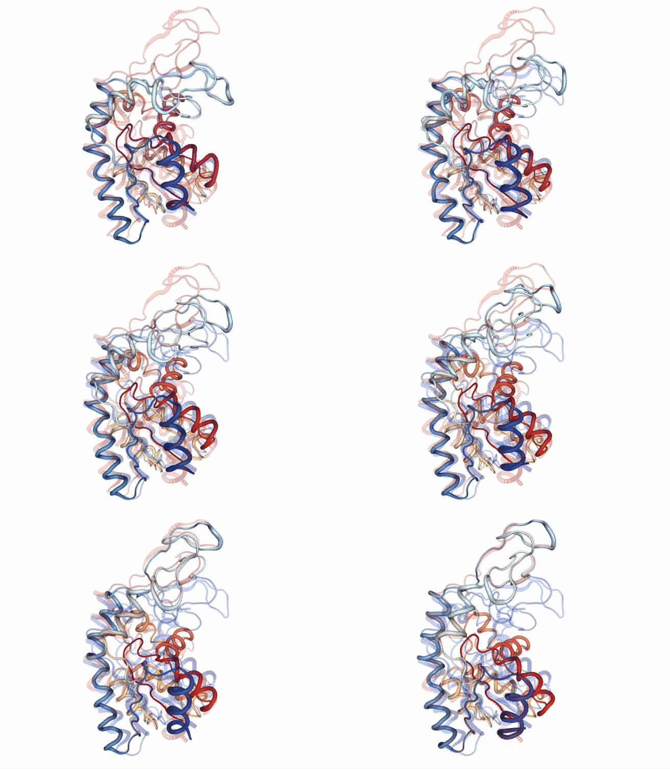
This tutorial aims to illustrate the process of computing a conformational transition between two known structural conformations of a protein, step by step, using the BioExcel Building Blocks library (biobb).

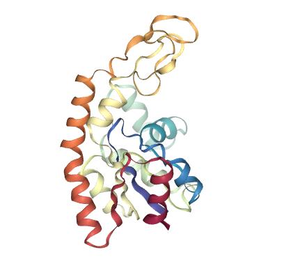
Examples shown are the calculation of the conformational transition for the Adenylate Kinase protein, from the closed state (PDB Code 1AKE, https://doi.org/10.2210/pdb1AKE/pdb) to the open state (PDB Code 4AKE, https://doi.org/10.2210/pdb4AKE/pdb). Adenylate Kinases are phosphotransferase enzymes that catalyze the interconversion of the various adenosine phosphates (ATP, ADP, and AMP), and are known to undergo large conformational changes during their catalytic cycle.

The code wrapped is the GOdMD method, developed in the Molecular Modeling and Bioinformatics group (IRB Barcelona). GOdMD determines pathways for conformational transitions in macromolecules using discrete molecular dynamics and biasing techniques based on a combination of essential dynamics and Maxwell-Demon sampling techniques. A web implementation of the method can be found here: https://mmb.irbbarcelona.org/GOdMD/index.php

Exploration of conformational transition pathways from coarse-grained simulations.
Sfriso P, Hospital A, Emperador A, Orozco M.
Bioinformatics, 129(16):1980-6.
Available at: https://doi.org/10.1093/bioinformatics/btt324

Settings

Biobb modules used

biobb_godmd: Tools to compute protein conformational transitions using GOdMD.
biobb_io: Tools to fetch biomolecular data from public databases.
biobb_structure_utils: Tools to modify or extract information from a PDB structure.
biobb_analysis: Tools to analyse Molecular Dynamics trajectories.

Auxiliary libraries used

emboss: Software that automatically copes with data in a variety of formats and even allows transparent retrieval of sequence data from the web.
jupyter: Free software, open standards, and web services for interactive computing across all programming languages.
plotly: Python interactive graphing library integrated in Jupyter notebooks.
nglview: Jupyter/IPython widget to interactively view molecular structures and trajectories in notebooks.
simpletraj: Lightweight coordinate-only trajectory reader based on code from GROMACS, MDAnalysis and VMD.

Conda Installation and Launch

git clone https://github.com/bioexcel/biobb_wf_godmd.git
cd biobb_wf_godmd
conda env create -f conda_env/environment.yml
conda activate biobb_wf_godmd
jupyter-notebook biobb_wf_godmd/notebooks/biobb_wf_godmd.ipynb

Initializing colab

The two cells below are used only in case this notebook is executed via Google Colab. Take into account that, for running conda on Google Colab, the condacolab library must be installed. As explained here, the installation requires a kernel restart, so when running this notebook in Google Colab, don't run all cells until this installation is properly finished and the kernel has restarted.

In [ ]:

# Only executed when using google colab
import sys
if 'google.colab' in sys.modules:
  import subprocess
  from pathlib import Path
  try:
    subprocess.run(["conda", "-V"], check=True)
  except FileNotFoundError:
    subprocess.run([sys.executable, "-m", "pip", "install", "condacolab"], check=True)
    import condacolab
    condacolab.install()
    # Clone repository
    repo_URL = "https://github.com/bioexcel/biobb_wf_godmd.git"
    repo_name = Path(repo_URL).name.split('.')[0]
    if not Path(repo_name).exists():
      subprocess.run(["mamba", "install", "-y", "git"], check=True)
      subprocess.run(["git", "clone", repo_URL], check=True)
      print("⏬ Repository properly cloned.")
    # Install environment
    print("⏳ Creating environment...")
    env_file_path = f"{repo_name}/conda_env/environment.yml"
    subprocess.run(["mamba", "env", "update", "-n", "base", "-f", env_file_path], check=True)
    print("🎨 Install NGLView dependencies...")
    subprocess.run(["mamba", "install", "-y", "-c", "conda-forge", "nglview==3.0.8", "ipywidgets=7.7.2"], check=True)
    print("👍 Conda environment successfully created and updated.")

In [ ]:

# Enable widgets for colab
if 'google.colab' in sys.modules:
  from google.colab import output
  output.enable_custom_widget_manager()
  # Change working dir
  import os
  os.chdir("biobb_wf_godmd/biobb_wf_godmd/notebooks")
  print(f"📂 New working directory: {os.getcwd()}")

Input parameters

Input parameters needed:

y libraries: Libraries to be used in the workflow are imported once at the beginning
pdbOrigin: PDB code for the origin structure (e.g. 1AKE, https://doi.org/10.2210/pdb1AKE/pdb)
chainOrigin: Chain for the origin structure (e.g. A)
ligandOrigin: Ligand (if present) for the origin structure (e.g. AP5, Drugbank DB01717)
pdbTarget: PDB code for the target structure (e.g. 4AKE, https://doi.org/10.2210/pdb4AKE/pdb)
chainTarget: Chain for the target structure (e.g. A)
ligandTarget: Ligand (if present) for the target structure (e.g. None)

In [ ]:

import os
import plotly
import plotly.graph_objs as go
import nglview
import ipywidgets

# Adenylate Kinase (ADK)
pdbOrigin = "1ake" 
chainOrigin = "A"
ligandOrigin = "AP5"

pdbTarget = "4ake" 
chainTarget = "A"
ligandTarget = None

# Other Examples (taken from https://mmb.irbbarcelona.org/TransAtlas/)

# Estrogen Receptor Alpha (ERα)
# pdbOrigin = "1a52" 
# pdbTarget = "3dt3" 
# chainOrigin = "A"
# chainTarget = "B"
# ligandOrigin = "EST"
# ligandTarget = "369"

# Calmodulin (CaM)
# pdbOrigin = "1deg" 
# pdbTarget = "2f2o" 
# chainOrigin = "A"
# chainTarget = "A"
# ligandOrigin = None
# ligandTarget = None

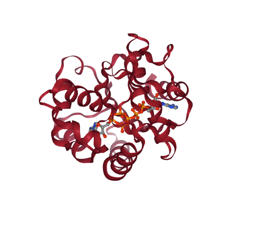
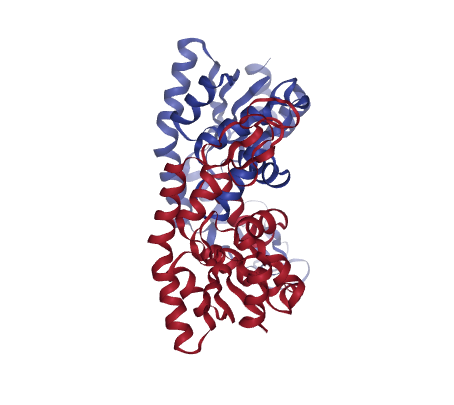
Fetching PDB structures

Downloading PDB structures with the origin and target protein molecules from the RCSB PDB database.
Alternatively, PDB files can be used as starting structures.

Building Blocks used:

Pdb from biobb_io.api.pdb

In [ ]:

# Import module
from biobb_io.api.pdb import pdb

# Create properties dict and inputs/outputs
originPDB = pdbOrigin+'.pdb'
targetPDB = pdbTarget+'.pdb'

prop_origin = {
    'pdb_code': pdbOrigin,
    'filter': False
}

prop_target = {
    'pdb_code': pdbTarget,
    'filter': False
}

# Launch bb for Origin PDB
pdb(output_pdb_path=originPDB,
    properties=prop_origin)

# Launch bb for Target PDB
pdb(output_pdb_path=targetPDB,
    properties=prop_target)

Visualizing 3D structures

Visualizing the downloaded/given PDB structures using NGL:

In [ ]:

# Show different structures (for comparison)

view1 = nglview.show_structure_file(originPDB)
#view1.add_representation(repr_type='ball+stick')
view1._remote_call('setSize', target='Widget', args=['400px','400px'])
view1.camera='orthographic'
view1
view2 = nglview.show_structure_file(targetPDB)
#view2.add_representation(repr_type='ball+stick')
view2._remote_call('setSize', target='Widget', args=['400px','400px'])
view2.camera='orthographic'
view2
ipywidgets.HBox([view1, view2])

No description has been provided for this image

Preparing the structures

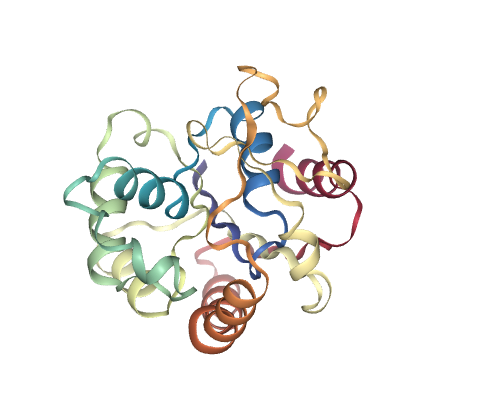
Preparing the structures to be used for the conformational transition calculation.

Extracting the interesting chains from the PDB structures (chain A in both cases).
Removing the inhibitor AP5A from the closed conformation.

Building Blocks used:

extract_chain from biobb_structure_utils.utils.extract_chain
remove_molecules from biobb_structure_utils.utils.remove_molecules

Extracting the interesting chains from the PDB structures (chain A in both cases).

In [ ]:

from biobb_structure_utils.utils.extract_chain import extract_chain

originPDB_chain = pdbOrigin + ".chains.pdb"
targetPDB_chain = pdbTarget + ".chains.pdb"

prop = {
    'chains': [ chainOrigin ]
}


# Launch bb for Origin PDB
extract_chain(
    input_structure_path=originPDB,
    output_structure_path=originPDB_chain,
    properties=prop
)

prop = {
    'chains': [ chainTarget ]
}

# Launch bb for Target PDB
extract_chain(
    input_structure_path=targetPDB,
    output_structure_path=targetPDB_chain,
    properties=prop
)

Removing the inhibitor AP5A from the closed conformation.

In [ ]:

from biobb_structure_utils.utils.remove_molecules import remove_molecules

originPDB_chain_nolig = pdbOrigin + ".chains.nolig.pdb"
targetPDB_chain_nolig = pdbTarget + ".chains.nolig.pdb"

if ligandOrigin:
    prop = {
        'molecules': [
            {
                'name' : ligandOrigin
            }
        ]
    }
    remove_molecules(input_structure_path=originPDB_chain,
                     output_molecules_path=originPDB_chain_nolig,
                     properties=prop)
else:
    originPDB_chain_nolig = originPDB_chain

if ligandTarget:
    prop = {
        'molecules': [
            {
                'name' : ligandTarget
            }
        ]
    }
    remove_molecules(input_structure_path=targetPDB_chain,
                     output_molecules_path=targetPDB_chain_nolig,
                     properties=prop)
else:
    targetPDB_chain_nolig = targetPDB_chain

Visualizing 3D structures

Visualizing the modified PDB structures using NGL:

In [ ]:

# Show different structures generated (for comparison)

view1 = nglview.show_structure_file(originPDB_chain_nolig)
#view1.add_representation(repr_type='ball+stick')
view1._remote_call('setSize', target='Widget', args=['400px','400px'])
view1.camera='orthographic'
view1
view2 = nglview.show_structure_file(targetPDB_chain_nolig)
#view2.add_representation(repr_type='ball+stick')
view2._remote_call('setSize', target='Widget', args=['400px','400px'])
view2.camera='orthographic'
view2
ipywidgets.HBox([view1, view2])

No description has been provided for this image

Computing the mapping

GOdMD works by moving the atoms from the position of the origin structure to the one in the target structure. For that, a one-to-one correspondance is needed. This step builds a couple of mapping files (.aln) from an internal sequence alignment (using EMBOSS water pairwise sequence alignment tool).

Building Blocks used:

godmd_prep from biobb_godmd.godmd.godmd_prep

In [ ]:

from biobb_godmd.godmd.godmd_prep import godmd_prep

originALN = pdbOrigin + ".aln"
targetALN = pdbTarget + ".aln"

prop = {
    'gapopen' : '12.0',
    'gapextend' : '2'
}

godmd_prep( input_pdb_orig_path=originPDB_chain_nolig,
            input_pdb_target_path=targetPDB_chain_nolig,
            output_aln_orig_path=originALN,
            output_aln_target_path=targetALN,
            properties=prop)

Running GOdMD

Computing the conformational transition, from the origin to the target structure, using GOdMD and the mappings generated in the previous step. The output file is a trajectory file in mdcrd format.

Building Blocks used:

godmd_run from biobb_godmd.godmd.godmd_run

In [ ]:

from biobb_godmd.godmd.godmd_run import godmd_run

godmd_log = pdbOrigin + "-" + pdbTarget + ".godmd.log"
godmd_trj = pdbOrigin + "-" + pdbTarget + ".godmd.mdcrd"
godmd_ene = pdbOrigin + "-" + pdbTarget + ".godmd.ene.out"
godmd_pdb = pdbOrigin + "-" + pdbTarget + ".godmd.pdb"

prop = {
    'godmdin':{
        'temp' : 400
    }
}

godmd_run(   input_pdb_orig_path=originPDB_chain_nolig,
             input_pdb_target_path=targetPDB_chain_nolig,
             input_aln_orig_path=originALN,
             input_aln_target_path=targetALN,
             output_log_path=godmd_log,
             output_ene_path=godmd_ene,
             output_trj_path=godmd_trj,
             output_pdb_path=godmd_pdb,
             properties=prop)

Converting trajectory to XTC (visualization)

Converting the generated GOdMD trajectory from the mdcrd format to a xtc format, for the sake of visualization with NGL (see next cell).

Building Blocks used:

cpptraj_convert from biobb_analysis.ambertools.cpptraj_convert

In [ ]:

from biobb_analysis.ambertools.cpptraj_convert import cpptraj_convert

godmd_trj_xtc = pdbOrigin + "-" + pdbTarget + ".godmd.xtc"

prop = {
    'format': 'xtc'
}

cpptraj_convert(input_top_path=godmd_pdb,
                input_traj_path=godmd_trj,
                output_cpptraj_path=godmd_trj_xtc,
                properties=prop)

Visualizing trajectory

Visualizing the GOdMD computed conformational transition using NGL. The scene shows the origin (tube, blue) and target (tube, red) structure for reference.

In [ ]:

# Show trajectory

view = nglview.show_simpletraj(nglview.SimpletrajTrajectory(godmd_trj_xtc, godmd_pdb), gui=True)

view.add_representation(repr_type='tube', colorScheme = 'atomindex')

# Origin Structure (comment when executing in google colab)
b = view.add_component(nglview.FileStructure(originPDB_chain_nolig))
b.clear_representations()
b.add_representation(repr_type='tube',
                        opacity=.2,
                        color='blue')

# Target Structure (comment when executing in google colab)
c = view.add_component(nglview.FileStructure(targetPDB_chain_nolig))
c.clear_representations()
c.add_representation(repr_type='tube', 
                       opacity=.2,
                        color='red')

# Align origin and target
code = """
var stage = this.stage;
var clist_len = stage.compList.length;
var i = 0;
var s = [];
for(i = 0; i <= clist_len; i++){
    if(stage.compList[i] != undefined && stage.compList[i].structure != undefined) {        
       s.push(stage.compList[i])
    }
}
NGL.superpose(s[1].structure, s[2].structure, true, ".CA")
s[ 1 ].updateRepresentations({ position: true })
s[ 1 ].autoView()
"""

#  (comment when executing in google colab)
view._execute_js_code(code)

view._remote_call('setSize', target='Widget', args=['800px','600px'])
view

No description has been provided for this image

Questions & Comments

Questions, issues, suggestions and comments are really welcome!

GitHub issues:
- https://github.com/bioexcel/biobb
BioExcel forum:
- https://ask.bioexcel.eu/c/BioExcel-Building-Blocks-library

Protein conformational transitions calculations

Protein Conformational Transitions calculations tutorial using BioExcel Building Blocks (biobb) and GOdMD

Settings

Biobb modules used

Auxiliary libraries used

Conda Installation and Launch

Pipeline steps

Initializing colab

Input parameters

Fetching PDB structures

Visualizing 3D structures

Preparing the structures

Visualizing 3D structures

Computing the mapping

Running GOdMD

Converting trajectory to XTC (visualization)

Visualizing trajectory

Questions & Comments