Protein MD Setup tutorial using BioExcel Building Blocks (biobb) through REST API

Based on the official GROMACS tutorial: https://www.mdtutorials.com/gmx/lysozyme/index.html

This tutorial aims to illustrate the process of setting up a simulation system containing a protein, step by step, using the BioExcel Building Blocks (biobb) REST API. The particular example used is the Lysozyme protein (PDB code 1AKI).

Settings

Auxiliar libraries used

requests: Requests allows you to send organic, grass-fed HTTP/1.1 requests, without the need for manual labor.
nb_conda_kernels: Enables a Jupyter Notebook or JupyterLab application in one conda environment to access kernels for Python, R, and other languages found in other environments.
nglview: Jupyter/IPython widget to interactively view molecular structures and trajectories in notebooks.
ipywidgets: Interactive HTML widgets for Jupyter notebooks and the IPython kernel.
plotly: Python interactive graphing library integrated in Jupyter notebooks.
simpletraj: Lightweight coordinate-only trajectory reader based on code from GROMACS, MDAnalysis and VMD.

Conda Installation and Launch

git clone https://github.com/bioexcel/biobb_wf_md_setup_api.git
 cd biobb_wf_md_setup_api
 conda env create -f conda_env/environment.yml
 conda activate biobb_MDsetupAPI_tutorial
 jupyter-nbextension enable --py --user widgetsnbextension
 jupyter-nbextension enable --py --user nglview
 jupyter-notebook biobb_wf_md_setup_api/notebooks/biobb_MDsetupAPI_tutorial.ipynb

Pipeline steps

Input Parameters
Fetching PDB Structure
Fix Protein Structure
Create Protein System Topology
Create Solvent Box
Fill the Box with Water Molecules
Adding Ions
Energetically Minimize the System
Equilibrate the System (NVT)
Equilibrate the System (NPT)
Free Molecular Dynamics Simulation
Post-processing and Visualizing Resulting 3D Trajectory
Output Files
Questions & Comments

Bioexcel2 logo

Input parameters

Input parameters needed:

pdbCode: PDB code of the protein structure (e.g. 1AKI)
apiURL: Base URL for the Biobb REST API (https://mmb.irbbarcelona.org/biobb-api/rest/v1/)

Additionally, the utils library is loaded. This library contains global functions that are used for sending and retrieving data to / from the REST API. Click here for more information about how the BioBB REST API works and which is the purpose for each of these functions.

import nglview
import ipywidgets
from utils import *

pdbCode = "1AKI"
apiURL  = "https://mmb.irbbarcelona.org/biobb-api/rest/v1/"

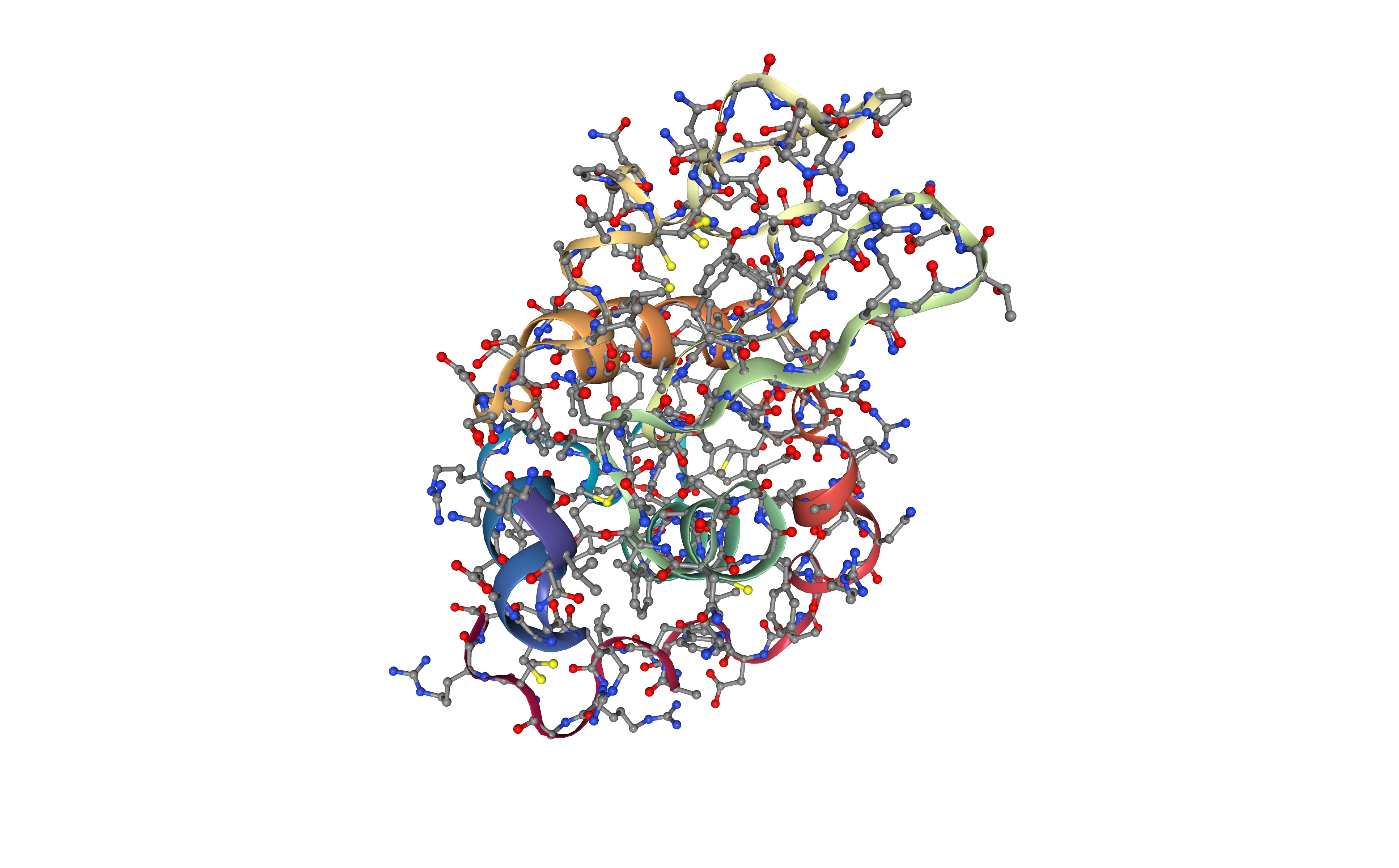
Fetching PDB structure

Downloading PDB structure with the protein molecule from the RCSB PDB database.
Alternatively, a PDB file can be used as starting structure.

BioBB REST API end points used:

PDB from biobb_io.api.pdb

# Downloading desired PDB file

# Create properties dict and inputs/outputs
downloaded_pdb = pdbCode + '.pdb'
prop = {
    'pdb_code': pdbCode
}

# Launch bb on REST API
token = launch_job(url = apiURL + 'launch/biobb_io/pdb', 
                   config = prop,
                   output_pdb_path = downloaded_pdb)

# Check job status
out_files = check_job(token, apiURL)

# Save generated file to disk
retrieve_data(out_files, apiURL)

Visualizing 3D structure

Visualizing the downloaded/given PDB structure using NGL:

# Show protein
view = nglview.show_structure_file(downloaded_pdb)
view.add_representation(repr_type='ball+stick', selection='all')
view._remote_call('setSize', target='Widget', args=['','600px'])
view

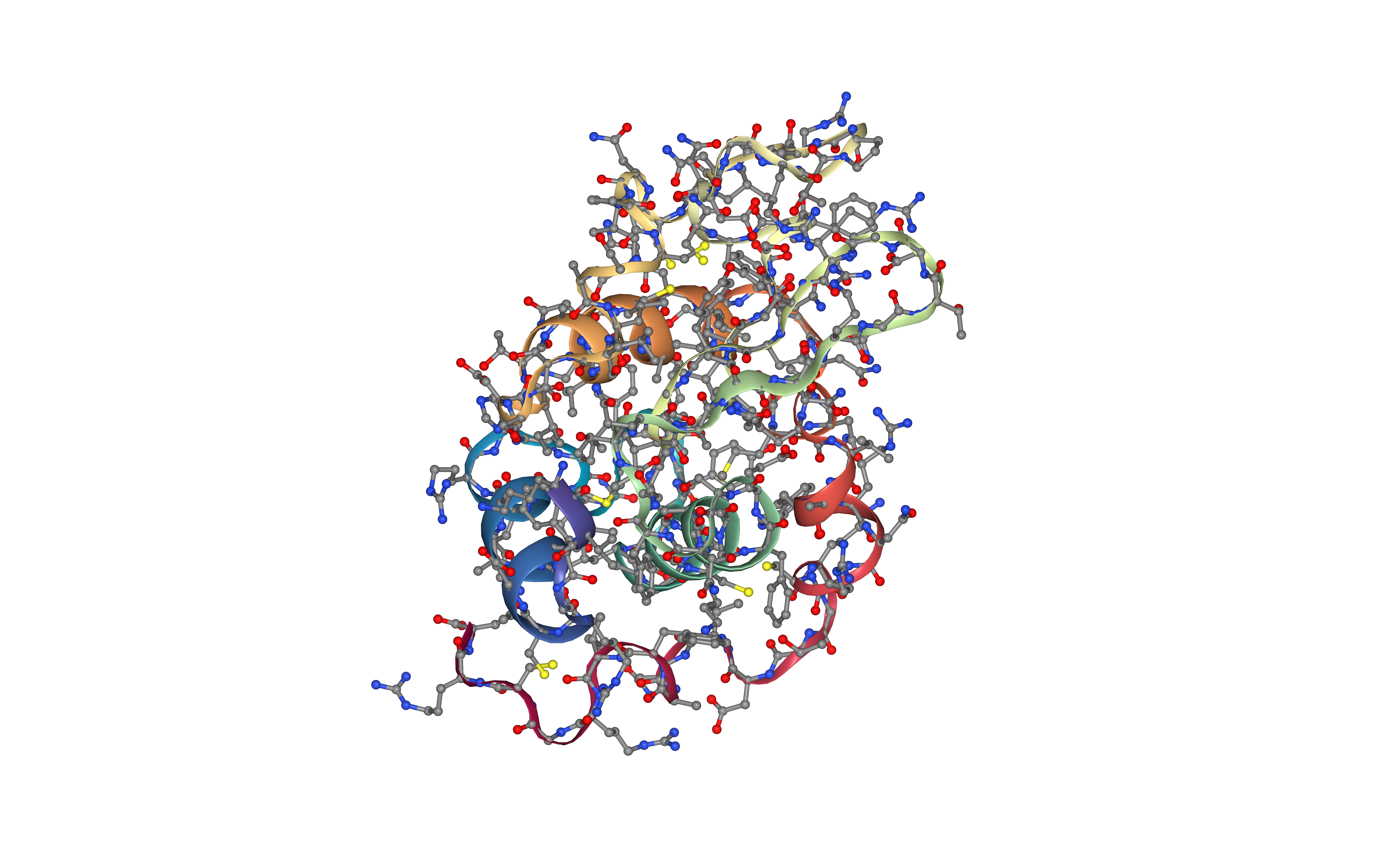
Fix protein structure

Checking and fixing (if needed) the protein structure:

Modeling missing side-chain atoms, modifying incorrect amide assignments, choosing alternative locations.
Checking for missing backbone atoms, heteroatoms, modified residues and possible atomic clashes.

BioBB REST API end points used:

FixSideChain from biobb_model.model.fix_side_chain

# Check & Fix PDB

# Create inputs/outputs
fixed_pdb = pdbCode + '_fixed.pdb'

# Launch bb on REST API
token = launch_job(url = apiURL + 'launch/biobb_model/fix_side_chain',
                   input_pdb_path = downloaded_pdb,
                   output_pdb_path = fixed_pdb)

# Check job status
out_files = check_job(token, apiURL)

# Save generated file to disk
retrieve_data(out_files, apiURL)

Visualizing 3D structure

Visualizing the fixed PDB structure using NGL. In this particular example, the checking step didn't find any issue to be solved, so there is no difference between the original structure and the fixed one.

# Show protein
view = nglview.show_structure_file(fixed_pdb)
view.add_representation(repr_type='ball+stick', selection='all')
view._remote_call('setSize', target='Widget', args=['','600px'])
view.camera='orthographic'
view

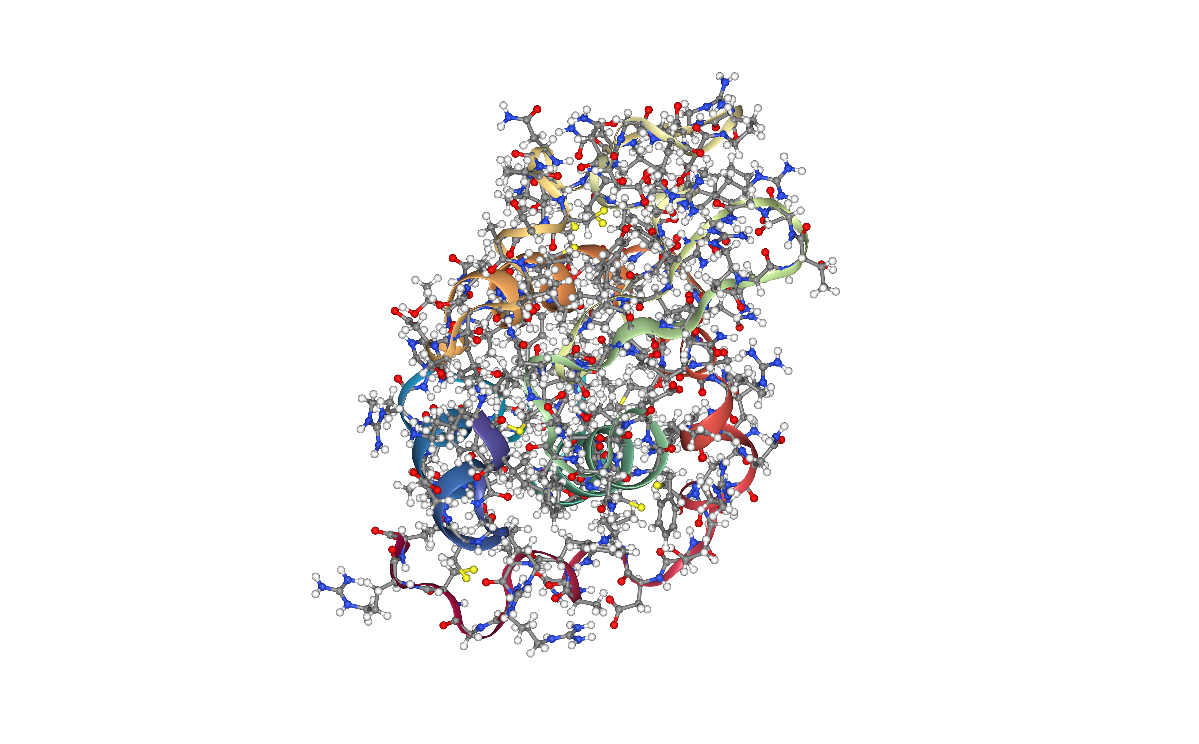
Create protein system topology

Building GROMACS topology corresponding to the protein structure.
Force field used in this tutorial is amber99sb-ildn: AMBER parm99 force field with corrections on backbone (sb) and side-chain torsion potentials (ildn). Water molecules type used in this tutorial is spc/e.
Adding hydrogen atoms if missing. Automatically identifying disulfide bridges.

Generating two output files:

GROMACS structure (gro file)
GROMACS topology ZIP compressed file containing:
- GROMACS topology top file (top file)
- GROMACS position restraint file/s (itp file/s)

BioBB REST API end points used:

Pdb2gmx from biobb_md.gromacs.pdb2gmx

# Create system topology

# Create inputs/outputs
output_pdb2gmx_gro = pdbCode + '_pdb2gmx.gro'
output_pdb2gmx_top_zip = pdbCode + '_pdb2gmx_top.zip'

# Launch bb on REST API
token = launch_job(url = apiURL + 'launch/biobb_md/pdb2gmx', 
                   input_pdb_path = fixed_pdb,
                   output_gro_path = output_pdb2gmx_gro,
                   output_top_zip_path = output_pdb2gmx_top_zip)

# Check job status
out_files = check_job(token, apiURL)

# Save generated file to disk
retrieve_data(out_files, apiURL)

Visualizing 3D structure

Visualizing the generated GRO structure using NGL. Note that hydrogen atoms were added to the structure by the pdb2gmx GROMACS tool when generating the topology.

# Show protein
view = nglview.show_structure_file(output_pdb2gmx_gro)
view.add_representation(repr_type='ball+stick', selection='all')
view._remote_call('setSize', target='Widget', args=['','600px'])
view.camera='orthographic'
view

Create solvent box

Define the unit cell for the protein structure MD system to fill it with water molecules.
A cubic box is used to define the unit cell, with a distance from the protein to the box edge of 1.0 nm. The protein is centered in the box.

BioBB REST API end points used:

Editconf from biobb_md.gromacs.editconf

# Editconf: Create solvent box

# Create properties dict and inputs/outputs
output_editconf_gro = pdbCode + '_editconf.gro'
prop = {
    'box_type': 'cubic',
    'distance_to_molecule': 1.0
}

# Launch bb on REST API
token = launch_job(url = apiURL + 'launch/biobb_md/editconf', 
                   config = prop,
                   input_gro_path = output_pdb2gmx_gro,
                   output_gro_path = output_editconf_gro)

# Check job status
out_files = check_job(token, apiURL)

# Save generated file to disk
retrieve_data(out_files, apiURL)

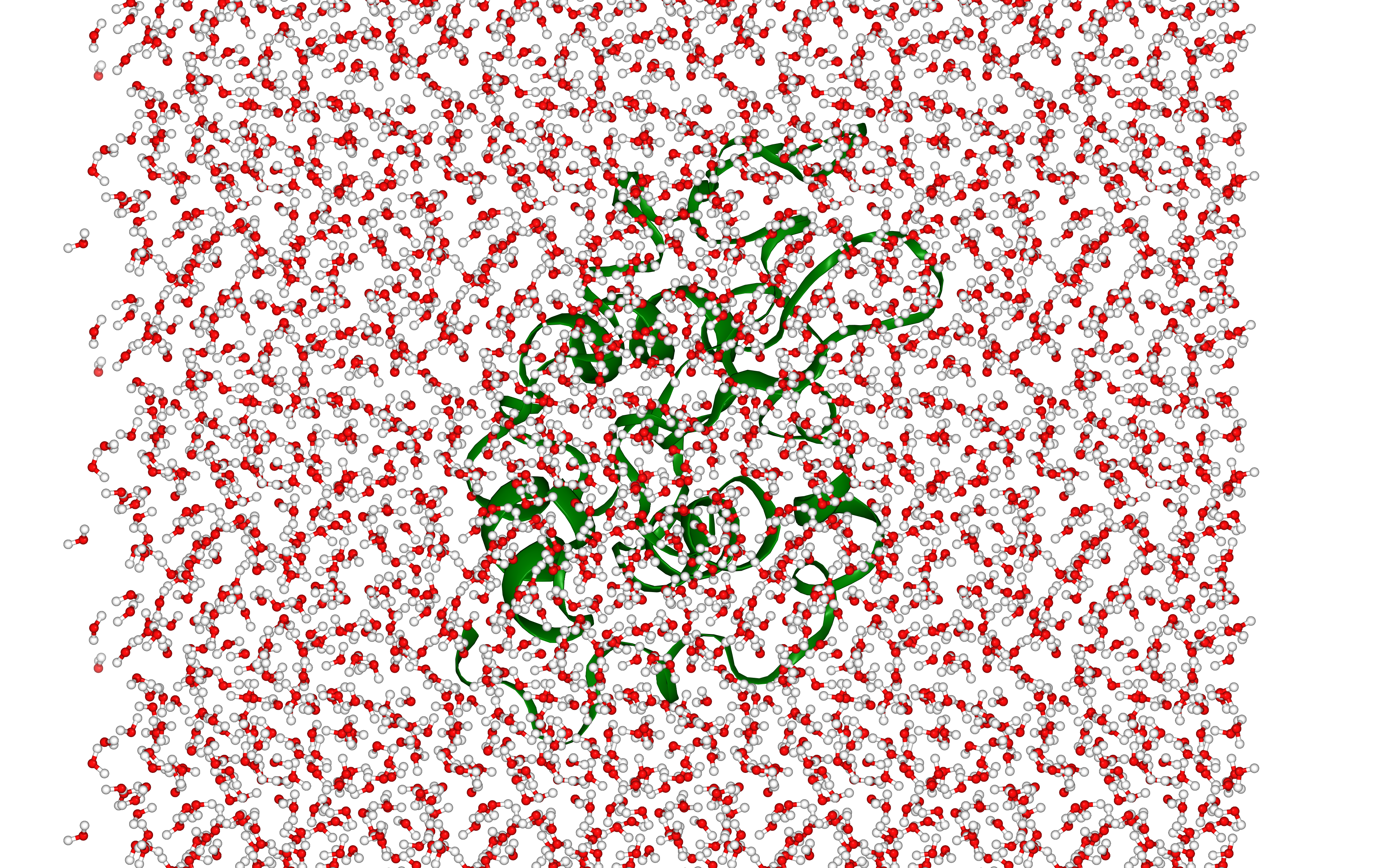
Fill the box with water molecules

Fill the unit cell for the protein structure system with water molecules.
The solvent type used is the default Simple Point Charge water (SPC), a generic equilibrated 3-point solvent model.

BioBB REST API end points used:

Solvate from biobb_md.gromacs.solvate

# Solvate: Fill the box with water molecules

# Create inputs/outputs
output_solvate_gro = pdbCode + '_solvate.gro'
output_solvate_top_zip = pdbCode + '_solvate_top.zip'

# Launch bb on REST API
token = launch_job(url = apiURL + 'launch/biobb_md/solvate', 
                   input_solute_gro_path = output_editconf_gro,
                   input_top_zip_path = output_pdb2gmx_top_zip,
                   output_gro_path = output_solvate_gro,
                   output_top_zip_path = output_solvate_top_zip)

# Check job status
out_files = check_job(token, apiURL)

# Save generated file to disk
retrieve_data(out_files, apiURL)

Visualizing 3D structure

Visualizing the protein system with the newly added solvent box using NGL.
Note the cubic box filled with water molecules surrounding the protein structure, which is centered right in the middle of the cube.

# Show protein
view = nglview.show_structure_file(output_solvate_gro)
view.clear_representations()
view.add_representation(repr_type='cartoon', selection='solute', color='green')
view.add_representation(repr_type='ball+stick', selection='SOL')
view._remote_call('setSize', target='Widget', args=['','600px'])
view.camera='orthographic'
view

Adding ions

Add ions to neutralize the protein structure charge

Step 1: Creating portable binary run file for ion generation
Step 2: Adding ions to neutralize the system

BioBB REST API end points used:

Grompp from biobb_md.gromacs.grompp
Genion from biobb_md.gromacs.genion

Step 1: Creating portable binary run file for ion generation

A simple energy minimization molecular dynamics parameters (mdp) properties will be used to generate the portable binary run file for ion generation, although any legitimate combination of parameters could be used in this step.

# Grompp: Creating portable binary run file for ion generation

# Create prop dict and inputs/outputs
output_gppion_tpr = pdbCode + '_gppion.tpr'
prop = {
    'simulation_type': 'minimization'
}

# Launch bb on REST API
token = launch_job(url = apiURL + 'launch/biobb_md/grompp', 
                   config = prop,
                   input_gro_path = output_solvate_gro,
                   input_top_zip_path = output_solvate_top_zip,
                   output_tpr_path = output_gppion_tpr)

# Check job status
out_files = check_job(token, apiURL)

# Save generated file to disk
retrieve_data(out_files, apiURL)

Step 2: Adding ions to neutralize the system

Replace solvent molecules with ions to neutralize the system.

# Genion: Adding ions to neutralize the system

# Create prop dict and inputs/outputs
output_genion_gro = pdbCode + '_genion.gro'
output_genion_top_zip = pdbCode + '_genion_top.zip'
prop={
    'neutral':True
}

# Launch bb on REST API
token = launch_job(url = apiURL + 'launch/biobb_md/genion',
                   config = prop,
                   input_tpr_path = output_gppion_tpr,
                   input_top_zip_path = output_solvate_top_zip,
                   output_gro_path = output_genion_gro,
                   output_top_zip_path = output_genion_top_zip)

# Check job status
out_files = check_job(token, apiURL)

# Save generated file to disk
retrieve_data(out_files, apiURL)

Visualizing 3D structure

Visualizing the neutralized protein system with the newly added ions using NGL

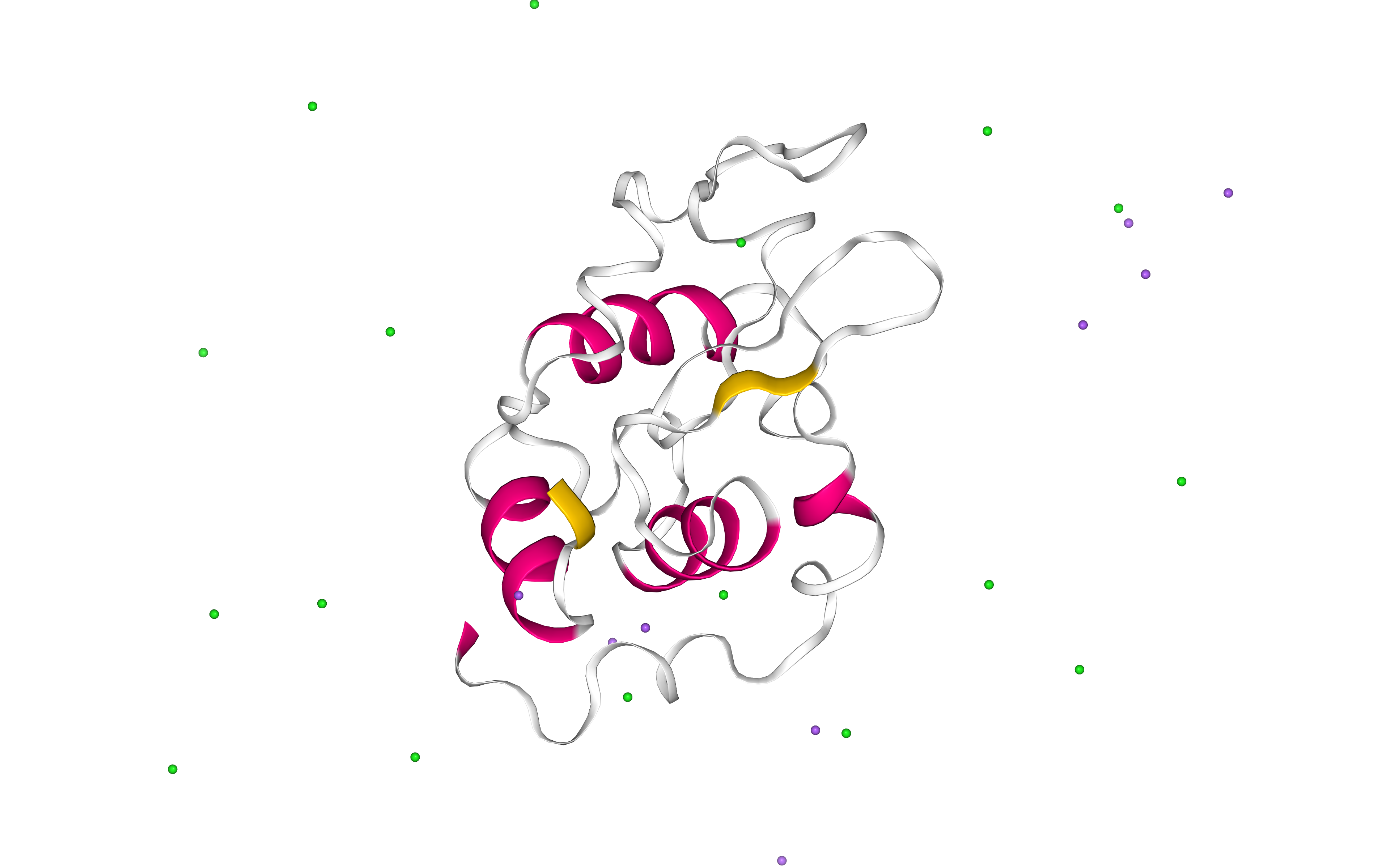
# Show protein
view = nglview.show_structure_file(output_genion_gro)
view.clear_representations()
view.add_representation(repr_type='cartoon', selection='solute', color='sstruc')
view.add_representation(repr_type='ball+stick', selection='NA')
view.add_representation(repr_type='ball+stick', selection='CL')
view._remote_call('setSize', target='Widget', args=['','600px'])
view.camera='orthographic'
view

Energetically minimize the system

Energetically minimize the protein system till reaching a desired potential energy.

Step 1: Creating portable binary run file for energy minimization
Step 2: Energetically minimize the system till reaching a force of 500 kJ mol-1 nm-1.
Step 3: Checking energy minimization results. Plotting energy by time during the minimization process.

BioBB REST API end points used:

Grompp from biobb_md.gromacs.grompp
Mdrun from biobb_md.gromacs.mdrun
GMXEnergy from biobb_analysis.gromacs.gmx_energy

Step 1: Creating portable binary run file for energy minimization

The minimization type of the molecular dynamics parameters (mdp) property contains the main default parameters to run an energy minimization:

integrator = steep ; Algorithm (steep = steepest descent minimization)
emtol = 1000.0 ; Stop minimization when the maximum force < 1000.0 kJ/mol/nm
emstep = 0.01 ; Minimization step size (nm)
nsteps = 50000 ; Maximum number of (minimization) steps to perform

In this particular example, the method used to run the energy minimization is the default steepest descent, but the maximum force is placed at 500 KJ/mol*nm^2, and the maximum number of steps to perform (if the maximum force is not reached) to 5,000 steps.

# Grompp: Creating portable binary run file for mdrun

# Create prop dict and inputs/outputs
output_gppmin_tpr = pdbCode + '_gppmin.tpr'
prop = {
    'mdp':{
        'emtol':'500',
        'nsteps':'5000'
    },
    'simulation_type': 'minimization'
}

# Launch bb on REST API
token = launch_job(url = apiURL + 'launch/biobb_md/grompp', 
                   config = prop,
                   input_gro_path = output_genion_gro,
                   input_top_zip_path = output_genion_top_zip,
                   output_tpr_path = output_gppmin_tpr)

# Check job status
out_files = check_job(token, apiURL)

# Save generated file to disk
retrieve_data(out_files, apiURL)

Step 2: Running Energy Minimization

Running energy minimization using the tpr file generated in the previous step.

# Mdrun: Running minimization

# Create inputs/outputs
output_min_trr = pdbCode + '_min.trr'
output_min_gro = pdbCode + '_min.gro'
output_min_edr = pdbCode + '_min.edr'
output_min_log = pdbCode + '_min.log'

# Launch bb on REST API
token = launch_job(url = apiURL + 'launch/biobb_md/mdrun', 
                   input_tpr_path = output_gppmin_tpr,
                   output_trr_path = output_min_trr,
                   output_gro_path = output_min_gro,
                   output_edr_path = output_min_edr,
                   output_log_path = output_min_log)

# Check job status
out_files = check_job(token, apiURL)

# Save generated file to disk
retrieve_data(out_files, apiURL)

Step 3: Checking Energy Minimization results

Checking energy minimization results. Plotting potential energy by time during the minimization process.

# GMXEnergy: Getting system energy by time 

# Create prop dict and inputs/outputs
output_min_ene_xvg = pdbCode + '_min_ene.xvg'
prop = {
    'terms':  ["Potential"]
}

# Launch bb on REST API
token = launch_job(url = apiURL + 'launch/biobb_analysis/gmx_energy',
                   config = prop,
                   input_energy_path = output_min_edr,
                   output_xvg_path = output_min_ene_xvg)

# Check job status
out_files = check_job(token, apiURL)

# Save generated file to disk
retrieve_data(out_files, apiURL)

import plotly
import plotly.graph_objs as go

#Read data from file and filter energy values higher than 1000 Kj/mol^-1
with open(output_min_ene_xvg,'r') as energy_file:
    x,y = map(
        list,
        zip(*[
            (float(line.split()[0]),float(line.split()[1]))
            for line in energy_file 
            if not line.startswith(("#","@")) 
            if float(line.split()[1]) < 1000 
        ])
    )

plotly.offline.init_notebook_mode(connected=True)

fig = {
    "data": [go.Scatter(x=x, y=y)],
    "layout": go.Layout(title="Energy Minimization",
                        xaxis=dict(title = "Energy Minimization Step"),
                        yaxis=dict(title = "Potential Energy KJ/mol-1")
                       )
}

plotly.offline.iplot(fig)

Equilibrate the system (NVT)

Equilibrate the protein system in NVT ensemble (constant Number of particles, Volume and Temperature). Protein heavy atoms will be restrained using position restraining forces: movement is permitted, but only after overcoming a substantial energy penalty. The utility of position restraints is that they allow us to equilibrate our solvent around our protein, without the added variable of structural changes in the protein.

Step 1: Creating portable binary run file for system equilibration
Step 2: Equilibrate the protein system with NVT ensemble.
Step 3: Checking NVT Equilibration results. Plotting system temperature by time during the NVT equilibration process.

BioBB REST API end points used:

Grompp from biobb_md.gromacs.grompp
Mdrun from biobb_md.gromacs.mdrun
GMXEnergy from biobb_analysis.gromacs.gmx_energy

Step 1: Creating portable binary run file for system equilibration (NVT)

The nvt type of the molecular dynamics parameters (mdp) property contains the main default parameters to run an NVT equilibration with protein restraints (see GROMACS mdp options):

Define = -DPOSRES
integrator = md
dt = 0.002
nsteps = 5000
pcoupl = no
gen_vel = yes
gen_temp = 300
gen_seed = -1

In this particular example, the default parameters will be used: md integrator algorithm, a step size of 2fs, 5,000 equilibration steps with the protein heavy atoms restrained, and a temperature of 300K.

Please note that for the sake of time this tutorial is only running 10ps of NVT equilibration, whereas in the original example the simulated time was 100ps.

# Grompp: Creating portable binary run file for NVT Equilibration

# Create prop dict and inputs/outputs
output_gppnvt_tpr = pdbCode + '_gppnvt.tpr'
prop = {
    'mdp':{
        'nsteps': 5000,
        'dt': 0.002,
        'Define': '-DPOSRES',
        #'tc_grps': "DNA Water_and_ions" # NOTE: uncomment this line if working with DNA
    },
    'simulation_type': 'nvt'
}

# Launch bb on REST API
token = launch_job(url = apiURL + 'launch/biobb_md/grompp',
                   config = prop,
                   input_gro_path = output_min_gro,
                   input_top_zip_path = output_genion_top_zip,
                   output_tpr_path = output_gppnvt_tpr)

# Check job status
out_files = check_job(token, apiURL)

# Save generated file to disk
retrieve_data(out_files, apiURL)

Step 2: Running NVT equilibration

Running energy minimization using the tpr file generated in the previous step.

# Mdrun: Running Equilibration NVT

# Create inputs/outputs
output_nvt_trr = pdbCode + '_nvt.trr'
output_nvt_gro = pdbCode + '_nvt.gro'
output_nvt_edr = pdbCode + '_nvt.edr'
output_nvt_log = pdbCode + '_nvt.log'
output_nvt_cpt = pdbCode + '_nvt.cpt'

# Launch bb on REST API
token = launch_job(url = apiURL + 'launch/biobb_md/mdrun',
                   input_tpr_path = output_gppnvt_tpr,
                   output_trr_path = output_nvt_trr,
                   output_gro_path = output_nvt_gro,
                   output_edr_path = output_nvt_edr,
                   output_log_path = output_nvt_log,
                   output_cpt_path = output_nvt_cpt)

# Check job status
out_files = check_job(token, apiURL)

# Save generated file to disk
retrieve_data(out_files, apiURL)

Step 3: Checking NVT Equilibration results

Checking NVT Equilibration results. Plotting system temperature by time during the NVT equilibration process.

# GMXEnergy: Getting system temperature by time during NVT Equilibration 

# Create prop dict and inputs/outputs
output_nvt_temp_xvg = pdbCode + '_nvt_temp.xvg'
prop = {
    'terms':  ["Temperature"]
}

# Launch bb on REST API
token = launch_job(url = apiURL + 'launch/biobb_analysis/gmx_energy', 
                   config = prop,
                   input_energy_path = output_nvt_edr,
                   output_xvg_path = output_nvt_temp_xvg)

# Check job status
out_files = check_job(token, apiURL)

# Save generated file to disk
retrieve_data(out_files, apiURL)

import plotly
import plotly.graph_objs as go

# Read temperature data from file 
with open(output_nvt_temp_xvg,'r') as temperature_file:
    x,y = map(
        list,
        zip(*[
            (float(line.split()[0]),float(line.split()[1]))
            for line in temperature_file 
            if not line.startswith(("#","@")) 
        ])
    )

plotly.offline.init_notebook_mode(connected=True)

fig = {
    "data": [go.Scatter(x=x, y=y)],
    "layout": go.Layout(title="Temperature during NVT Equilibration",
                        xaxis=dict(title = "Time (ps)"),
                        yaxis=dict(title = "Temperature (K)")
                       )
}

plotly.offline.iplot(fig)

Equilibrate the system (NPT)

Equilibrate the protein system in NPT ensemble (constant Number of particles, Pressure and Temperature).

Step 1: Creating portable binary run file for system equilibration
Step 2: Equilibrate the protein system with NPT ensemble.
Step 3: Checking NPT Equilibration results. Plotting system pressure and density by time during the NPT equilibration process.

BioBB REST API end points used:

Grompp from biobb_md.gromacs.grompp
Mdrun from biobb_md.gromacs.mdrun
GMXEnergy from biobb_analysis.gromacs.gmx_energy

Step 1: Creating portable binary run file for system equilibration (NPT)

The npt type of the molecular dynamics parameters (mdp) property contains the main default parameters to run an NPT equilibration with protein restraints (see GROMACS mdp options):

Define = -DPOSRES
integrator = md
dt = 0.002
nsteps = 5000
pcoupl = Parrinello-Rahman
pcoupltype = isotropic
tau_p = 1.0
ref_p = 1.0
compressibility = 4.5e-5
refcoord_scaling = com
gen_vel = no

In this particular example, the default parameters will be used: md integrator algorithm, a time step of 2fs, 5,000 equilibration steps with the protein heavy atoms restrained, and a Parrinello-Rahman pressure coupling algorithm.

Please note that for the sake of time this tutorial is only running 10ps of NPT equilibration, whereas in the original example the simulated time was 100ps.

# Grompp: Creating portable binary run file for NPT System Equilibration

# Create prop dict and inputs/outputs
output_gppnpt_tpr = pdbCode + '_gppnpt.tpr'
prop = {
    'mdp':{
        'nsteps':'5000',
        #'tc_grps': "DNA Water_and_ions" # NOTE: uncomment this line if working with DNA
    },
    'simulation_type': 'npt'
}

# Launch bb on REST API
token = launch_job(url = apiURL + 'launch/biobb_md/grompp', 
                   config = prop,
                   input_gro_path = output_nvt_gro,
                   input_top_zip_path = output_genion_top_zip,
                   output_tpr_path = output_gppnpt_tpr)

# Check job status
out_files = check_job(token, apiURL)

# Save generated file to disk
retrieve_data(out_files, apiURL)

Step 2: Running NPT equilibration

# Mdrun: Running NPT System Equilibration

# Create inputs/outputs
output_npt_trr = pdbCode + '_npt.trr'
output_npt_gro = pdbCode + '_npt.gro'
output_npt_edr = pdbCode + '_npt.edr'
output_npt_log = pdbCode + '_npt.log'
output_npt_cpt = pdbCode + '_npt.cpt'

# Launch bb on REST API
token = launch_job(url = apiURL + 'launch/biobb_md/mdrun',
                   input_tpr_path = output_gppnpt_tpr,
                   output_trr_path = output_npt_trr,
                   output_gro_path = output_npt_gro,
                   output_edr_path = output_npt_edr,
                   output_log_path = output_npt_log,
                   output_cpt_path = output_npt_cpt)

# Check job status
out_files = check_job(token, apiURL)

# Save generated file to disk
retrieve_data(out_files, apiURL)

Step 3: Checking NPT Equilibration results

Checking NPT Equilibration results. Plotting system pressure and density by time during the NPT equilibration process.

# GMXEnergy: Getting system pressure and density by time during NPT Equilibration 

# Create prop dict and inputs/outputs
output_npt_pd_xvg = pdbCode + '_npt_PD.xvg'
prop = {
    'terms':  ["Pressure","Density"]
}

# Launch bb on REST API
token = launch_job(url = apiURL + 'launch/biobb_analysis/gmx_energy',
                   config = prop,
                   input_energy_path = output_npt_edr,
                   output_xvg_path = output_npt_pd_xvg)

# Check job status
out_files = check_job(token, apiURL)

# Save generated file to disk
retrieve_data(out_files, apiURL)

import plotly
from plotly import subplots
import plotly.graph_objs as go

# Read pressure and density data from file 
with open(output_npt_pd_xvg,'r') as pd_file:
    x,y,z = map(
        list,
        zip(*[
            (float(line.split()[0]),float(line.split()[1]),float(line.split()[2]))
            for line in pd_file 
            if not line.startswith(("#","@")) 
        ])
    )

plotly.offline.init_notebook_mode(connected=True)

trace1 = go.Scatter(
    x=x,y=y
)
trace2 = go.Scatter(
    x=x,y=z
)

fig = subplots.make_subplots(rows=1, cols=2, print_grid=False)

fig.append_trace(trace1, 1, 1)
fig.append_trace(trace2, 1, 2)

fig['layout']['xaxis1'].update(title='Time (ps)')
fig['layout']['xaxis2'].update(title='Time (ps)')
fig['layout']['yaxis1'].update(title='Pressure (bar)')
fig['layout']['yaxis2'].update(title='Density (Kg*m^-3)')

fig['layout'].update(title='Pressure and Density during NPT Equilibration')
fig['layout'].update(showlegend=False)

plotly.offline.iplot(fig)

Free Molecular Dynamics Simulation

Upon completion of the two equilibration phases (NVT and NPT), the system is now well-equilibrated at the desired temperature and pressure. The position restraints can now be released. The last step of the protein MD setup is a short, free MD simulation, to ensure the robustness of the system.

Step 1: Creating portable binary run file to run a free MD simulation.
Step 2: Run short MD simulation of the protein system.
Step 3: Checking results for the final step of the setup process, the free MD run. Plotting Root Mean Square deviation (RMSd) and Radius of Gyration (Rgyr) by time during the free MD run step.

BioBB REST API end points used:

Grompp from biobb_md.gromacs.grompp
Mdrun from biobb_md.gromacs.mdrun
GMXRms from biobb_analysis.gromacs.gmx_rms
GMXRgyr from biobb_analysis.gromacs.gmx_rgyr

Step 1: Creating portable binary run file to run a free MD simulation

The free type of the molecular dynamics parameters (mdp) property contains the main default parameters to run an free MD simulation (see GROMACS mdp options):

integrator = md
dt = 0.002 (ps)
nsteps = 50000

In this particular example, the default parameters will be used: md integrator algorithm, a time step of 2fs, and a total of 50,000 md steps (100ps).

Please note that for the sake of time this tutorial is only running 100ps of free MD, whereas in the original example the simulated time was 1ns (1000ps).

# Grompp: Creating portable binary run file for mdrun

# Create prop dict and inputs/outputs
output_gppmd_tpr = pdbCode + '_gppmd.tpr'
prop = {
    'mdp':{
        'nsteps':'50000',
        #'tc_grps': "DNA Water_and_ions" # NOTE: uncomment this line if working with DNA
    },
    'simulation_type': 'free'
}

# Launch bb on REST API
token = launch_job(url = apiURL + 'launch/biobb_md/grompp',
                   config = prop,
                   input_gro_path = output_npt_gro,
                   input_top_zip_path = output_genion_top_zip,
                   output_tpr_path = output_gppmd_tpr)

# Check job status
out_files = check_job(token, apiURL)

# Save generated file to disk
retrieve_data(out_files, apiURL)

Step 2: Running short free MD simulation

# Mdrun: Running free dynamics

# Create inputs/outputs
output_md_trr = pdbCode + '_md.trr'
output_md_gro = pdbCode + '_md.gro'
output_md_edr = pdbCode + '_md.edr'
output_md_log = pdbCode + '_md.log'
output_md_cpt = pdbCode + '_md.cpt'

# Launch bb on REST API
token = launch_job(url = apiURL + 'launch/biobb_md/mdrun',
                   input_tpr_path = output_gppmd_tpr,
                   output_trr_path = output_md_trr,
                   output_gro_path = output_md_gro,
                   output_edr_path = output_md_edr,
                   output_log_path = output_md_log,
                   output_cpt_path = output_md_cpt)

# Check job status
out_files = check_job(token, apiURL)

# Save generated file to disk
retrieve_data(out_files, apiURL)

Step 3: Checking free MD simulation results

Checking results for the final step of the setup process, the free MD run. Plotting Root Mean Square deviation (RMSd) and Radius of Gyration (Rgyr) by time during the free MD run step. RMSd against the experimental structure (input structure of the pipeline) and against the minimized and equilibrated structure (output structure of the NPT equilibration step).

# GMXRms: Computing Root Mean Square deviation to analyse structural stability 
#         RMSd against minimized and equilibrated snapshot (backbone atoms)  

# Create prop dict and inputs/outputs
output_rms_first = pdbCode + '_rms_first.xvg'
prop = {
    'selection':  'Backbone',
    #'selection': 'non-Water'
}

# Launch bb on REST API
token = launch_job(url = apiURL + 'launch/biobb_analysis/gmx_rms', 
                   config = prop,
                   input_structure_path = output_gppmd_tpr,
                   input_traj_path = output_md_trr,
                   output_xvg_path = output_rms_first)

# Check job status
out_files = check_job(token, apiURL)

# Save generated file to disk
retrieve_data(out_files, apiURL)

# GMXRms: Computing Root Mean Square deviation to analyse structural stability 
#         RMSd against experimental structure (backbone atoms)  

# Create prop dict and inputs/outputs
output_rms_exp = pdbCode + '_rms_exp.xvg'
prop = {
    'selection':  'Backbone',
    #'selection': 'non-Water'
}

# Launch bb on REST API
token = launch_job(url = apiURL + 'launch/biobb_analysis/gmx_rms',
                   config = prop,
                   input_structure_path = output_gppmin_tpr,
                   input_traj_path = output_md_trr,
                   output_xvg_path = output_rms_exp)

# Check job status
out_files = check_job(token, apiURL)

# Save generated file to disk
retrieve_data(out_files, apiURL)

import plotly
import plotly.graph_objs as go

# Read RMS vs first snapshot data from file 
with open(output_rms_first,'r') as rms_first_file:
    x,y = map(
        list,
        zip(*[
            (float(line.split()[0]),float(line.split()[1]))
            for line in rms_first_file 
            if not line.startswith(("#","@")) 
        ])
    )

# Read RMS vs experimental structure data from file 
with open(output_rms_exp,'r') as rms_exp_file:
    x2,y2 = map(
        list,
        zip(*[
            (float(line.split()[0]),float(line.split()[1]))
            for line in rms_exp_file
            if not line.startswith(("#","@")) 
        ])
    )
    
trace1 = go.Scatter(
    x = x,
    y = y,
    name = 'RMSd vs first'
)

trace2 = go.Scatter(
    x = x,
    y = y2,
    name = 'RMSd vs exp'
)

data = [trace1, trace2]

plotly.offline.init_notebook_mode(connected=True)

fig = {
    "data": data,
    "layout": go.Layout(title="RMSd during free MD Simulation",
                        xaxis=dict(title = "Time (ps)"),
                        yaxis=dict(title = "RMSd (nm)")
                       )
}

plotly.offline.iplot(fig)

# GMXRgyr: Computing Radius of Gyration to measure the protein compactness during the free MD simulation 

# Create prop dict and inputs/outputs
output_rgyr = pdbCode + '_rgyr.xvg'
prop = {
    'selection':  'Backbone'
}

# Launch bb on REST API
token = launch_job(url = apiURL + 'launch/biobb_analysis/gmx_rgyr', 
                   config = prop,
                   input_structure_path = output_gppmin_tpr,
                   input_traj_path = output_md_trr,
                   output_xvg_path = output_rgyr)

# Check job status
out_files = check_job(token, apiURL)

# Save generated file to disk
retrieve_data(out_files, apiURL)

import plotly
import plotly.graph_objs as go

# Read Rgyr data from file 
with open(output_rgyr,'r') as rgyr_file:
    x,y = map(
        list,
        zip(*[
            (float(line.split()[0]),float(line.split()[1]))
            for line in rgyr_file 
            if not line.startswith(("#","@")) 
        ])
    )

plotly.offline.init_notebook_mode(connected=True)

fig = {
    "data": [go.Scatter(x=x, y=y)],
    "layout": go.Layout(title="Radius of Gyration",
                        xaxis=dict(title = "Time (ps)"),
                        yaxis=dict(title = "Rgyr (nm)")
                       )
}

plotly.offline.iplot(fig)

Post-processing and Visualizing resulting 3D trajectory

Post-processing and Visualizing the protein system MD setup resulting trajectory using NGL

Step 1: Imaging the resulting trajectory, stripping out water molecules and ions and correcting periodicity issues.
Step 2: Generating a dry structure, removing water molecules and ions from the final snapshot of the MD setup pipeline.
Step 3: Visualizing the imaged trajectory using the dry structure as a topology.

BioBB REST API end points used:

GMXImage from biobb_analysis.gromacs.gmx_image
GMXTrjConvStr from biobb_analysis.gromacs.gmx_trjconv_str

Step 1: Imaging the resulting trajectory.

Stripping out water molecules and ions and correcting periodicity issues

# GMXImage: "Imaging" the resulting trajectory
#           Removing water molecules and ions from the resulting structure

# Create prop dict and inputs/outputs
output_imaged_traj = pdbCode + '_imaged_traj.trr'
prop = {
    'center_selection':  'Protein',
    'output_selection': 'Protein',
    'pbc' : 'mol',
    'center' : True
}

# Launch bb on REST API
token = launch_job(url = apiURL + 'launch/biobb_analysis/gmx_image',
                   config = prop,
                   input_traj_path = output_md_trr,
                   input_top_path = output_gppmd_tpr,
                   output_traj_path = output_imaged_traj)

# Check job status
out_files = check_job(token, apiURL)

# Save generated file to disk
retrieve_data(out_files, apiURL)

Step 2: Generating the output dry structure.

Removing water molecules and ions from the resulting structure

# GMXTrjConvStr: Converting and/or manipulating a structure
#                Removing water molecules and ions from the resulting structure
#                The "dry" structure will be used as a topology to visualize 
#                the "imaged dry" trajectory generated in the previous step.

# Create prop dict and inputs/outputs
output_dry_gro = pdbCode + '_md_dry.gro'
prop = {
    'selection':  'Protein'
}

# Launch bb on REST API
token = launch_job(url = apiURL + 'launch/biobb_analysis/gmx_trjconv_str',
                   config = prop,
                   input_structure_path = output_md_gro,
                   input_top_path = output_gppmd_tpr,
                   output_str_path = output_dry_gro)

# Check job status
out_files = check_job(token, apiURL)

# Save generated file to disk
retrieve_data(out_files, apiURL)

Step 3: Visualizing the generated dehydrated trajectory.

Using the imaged trajectory (output of the Post-processing step 1) with the dry structure (output of the Post-processing step 2) as a topology.

# Show trajectory
view = nglview.show_simpletraj(nglview.SimpletrajTrajectory(output_imaged_traj, output_dry_gro), gui=True)
view

Output files

Important Output files generated:

1AKI_md.gro: Final structure (snapshot) of the MD setup protocol.
1AKI_md.trr: Final trajectory of the MD setup protocol.
1AKI_md.cpt: Final checkpoint file, with information about the state of the simulation. It can be used to restart or continue a MD simulation.
1AKI_gppmd.tpr: Final tpr file, GROMACS portable binary run input file. This file contains the starting structure of the MD setup free MD simulation step, together with the molecular topology and all the simulation parameters. It can be used to extend the simulation.
1AKI_genion_top.zip: Final topology of the MD system. It is a compressed zip file including a topology file (.top) and a set of auxiliar include topology files (.itp).

Analysis (MD setup check) output files generated:

1AKI_rms_first.xvg: Root Mean Square deviation (RMSd) against minimized and equilibrated structure of the final free MD run step.
1AKI_rms_exp.xvg: Root Mean Square deviation (RMSd) against experimental structure of the final free MD run step.
1AKI_rgyr.xvg: Radius of Gyration of the final free MD run step of the setup pipeline.

Questions & Comments

Questions, issues, suggestions and comments are really welcome!

GitHub issues:
- https://github.com/bioexcel/biobb
BioExcel forum:
- https://ask.bioexcel.eu/c/BioExcel-Building-Blocks-library

Protein MD Setup tutorial using BioExcel Building Blocks through BioBB REST API

Protein MD Setup tutorial using BioExcel Building Blocks (biobb) through REST API

Settings

Auxiliar libraries used

Conda Installation and Launch

Pipeline steps

Input parameters

Fetching PDB structure

Visualizing 3D structure

Fix protein structure

Visualizing 3D structure

Create protein system topology

Visualizing 3D structure

Create solvent box

Fill the box with water molecules

Visualizing 3D structure

Adding ions

Step 1: Creating portable binary run file for ion generation

Step 2: Adding ions to neutralize the system

Visualizing 3D structure

Energetically minimize the system

Step 1: Creating portable binary run file for energy minimization

Step 2: Running Energy Minimization

Step 3: Checking Energy Minimization results

Equilibrate the system (NVT)

Step 1: Creating portable binary run file for system equilibration (NVT)

Step 2: Running NVT equilibration

Step 3: Checking NVT Equilibration results

Equilibrate the system (NPT)

Step 1: Creating portable binary run file for system equilibration (NPT)

Step 2: Running NPT equilibration

Step 3: Checking NPT Equilibration results

Free Molecular Dynamics Simulation

Step 1: Creating portable binary run file to run a free MD simulation

Step 2: Running short free MD simulation

Step 3: Checking free MD simulation results

Post-processing and Visualizing resulting 3D trajectory

Step 1: Imaging the resulting trajectory.

Step 2: Generating the output dry structure.

Step 3: Visualizing the generated dehydrated trajectory.

Output files

Questions & Comments