MC DNA Help - Analysis PCAZip

Principal Components

Method

Following Essential Dynamics algorithm (ED), the orthogonal movements describing the variance of a system trajectory is obtained by diagonalization of the covariance matrix.

The result of the analysis is the generation of a set of eigenvectors (the modes or the principal components), which describe the nature of the deformation movements of the protein and a set of eigenvalues, which indicate the stiffness associated to every mode.

The eigenvectors appear ranked after a principal component analysis, the first one is that explaining the largest part of the variance (as indicated by the associated eigenvalue). Since the eigenvectors represent a full-basis set the original Cartesian trajectory can be always projected into the eigenvectors space, without lost of information.

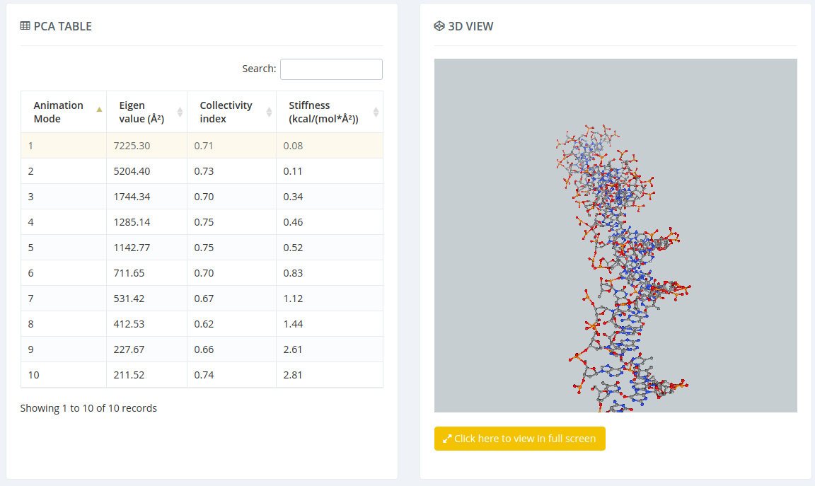
Each of the eigenvector obtained from Principal Component Analysis of a trajectory is called a Principal Component. The associated eigenvalue indicates the amount of variance explained by the component. The Collectivity Index gives a measure of how many atoms of the protein are affected by a Principal Component.

MC DNA uses PCAsuite package to compute Principal Components Flexibility Analysis. PCA is computed using all the atoms of the structure and the compression is reduced to a 90% of the explained variance. Only the first 10 principal components are shown in the graphical interface, as the first modes are usually the ones explaining the largest part of the variance.

Results

The Principal Component Analysis graphical interface offers the possibility of studying the real movements of the structure through the projections of the trajectory onto the different essential modes. An interactive NGL Viewer shows these movements, allowing user to translate, rotate and in general manipulate the visualization. The first 10 animation modes are offered for visualization and download. Associated values as eigenvalues, collectivity indexes and eigenvector stiffness constants are also shown.

For each of the first 10 eigenvectors, a plot containing the displacement (in Angstroms) of the projections of all the trajectory snapshots into the associated eigenvector from the first snapshot is also computed and shown. Plots generated contain the corresponding histogram attached, and an associated table with calculated mean and standard deviation values. Raw data and plot are also easily downloadable.